Session4.knit

class: center, middle, inverse, title-slide

# Single-cell RNA sequencing ~ Session 4
<html>
<div style="float:left">

</div>
<hr color='#EB811B' size=1px width=796px>
</html>
### Rockefeller University, Bioinformatics Resource Centre
### <a href="https://rockefelleruniversity.github.io/scRNA-seq/" class="uri">https://rockefelleruniversity.github.io/scRNA-seq/</a>

---

## Overview

So far we have used the Seurat and Bioconductor libraries to perform our single-cell RNA-seq analysis.

Python offers a range of libraries for the analysis of single-cell data.

Two of the most popular libraries for the analysis of single-cell RNA-seq are the [AnnData](https://anndata.readthedocs.io/en/latest/) and [scanpy](https://scanpy.readthedocs.io/en/stable/) packages.

---
## Scanpy Tutorial

In today's session we will follow the [scanpy tutorial](https://scanpy-tutorials.readthedocs.io/en/latest/pbmc3k.html) (which itself follows the [Seurat tutorial](https://satijalab.org/seurat/articles/pbmc3k_tutorial.html)..) and will implement all of the steps up to clustering and visualisation of clusters in a UMAP plot.

---
## Python from R

To make use of the AnnData and scanpy libraries we will need to work within a Python environment.

The reticulate package offers a method to use Python from within a R session and provides methods for the *silent* conversion between python and R objects.

---
class: inverse, center, middle

# Reticulate and python

---

## Install reticulate

Reticulate is maintained by Rstudio and is available from CRAN.

To install we can just run the standard **install.packages()** function and then load the library.

```r
install.packages("reticulate")
library(reticulate)
```

---
## Install Python from Conda

Once we have installed reticulate, we can then install Python.

To install python for reticulate we can make use of the install_miniconda() function. This will install conda into the default location as decided by reticulate.

For more option on installing python into specific directories, **?install_miniconda**.

```r
install_miniconda()
```

---
## Install Python packages

Just as with R libraries, we need to install the packages scanpy and AnnData into our Python library.

We can use the **conda_install()** function to install packages into our newly created conda environment.

Here we install the packages required for scRNA-seq analysis.

```r
conda_install(packages = c("python-igraph", "scanpy", "louvain", "leidenalg", "loompy"))
```

---
## Use conda python

Once we have installed Conda and the required python libraries into the conda enviroment, we can then set reticulate to use this python with the function **use_condaenv()**.

```r
use_condaenv()
py_config()
```

```
## python:         /github/home/.local/share/r-miniconda/envs/r-reticulate/bin/python
## libpython:      /github/home/.local/share/r-miniconda/envs/r-reticulate/lib/libpython3.6m.so
## pythonhome:     /github/home/.local/share/r-miniconda/envs/r-reticulate:/github/home/.local/share/r-miniconda/envs/r-reticulate
## version:        3.6.13 | packaged by conda-forge | (default, Feb 19 2021, 05:36:01)  [GCC 9.3.0]
## numpy:          /github/home/.local/share/r-miniconda/envs/r-reticulate/lib/python3.6/site-packages/numpy
## numpy_version:  1.19.5
```

---
## Conda python config

We can then check the versions of python in use by running the **py_config()** command.

This lists the python path, C/C++ library path as well as additional information on the install.

```r
use_condaenv()
py_config()
```

---
## Load python library

To load python libraries we will use reticulate's **import()** function. We just specify the python package to load and the object in R to load package to.

```r
sc <- reticulate::import("scanpy")
sc
```

```
## Module(scanpy)
```

---
## AnnData

The AnnData Python package offers a similar data structure to R/Bioconductor's SingleCellExperiment.

---
## Install anndata package

The CRAN anndata R package offers additional functionality for interacting with AnnData python objects on top of that offered by reticulate.

```r
install.packages("anndata")
library(anndata)
```

---
## anndata functionality

The anndata package allows us to interact with the complex python AnnData object much as if it was an R object.

This includes sub-setting and replacement within the AnnData object.

---
## Download PBMC

Before we start any analysis we will download the PBMC3K dataset from 10xgenomics website.

```r
pathToDownload <- "http://cf.10xgenomics.com/samples/cell-exp/1.1.0/pbmc3k/pbmc3k_filtered_gene_bc_matrices.tar.gz"
download.file(pathToDownload, "pbmc3k_filtered_gene_bc_matrices.tar.gz")
utils::untar("pbmc3k_filtered_gene_bc_matrices.tar.gz")
```

---
## Read PBMC

Now we have the data downloaded we can import into R/Python using the **read_10x_mtx()** function.

The result is a Python AnnData object.

```r
adata <- sc$read_10x_mtx("filtered_gene_bc_matrices/hg19/", var_names = "gene_ids")

adata
```

```
## AnnData object with n_obs × n_vars = 2700 × 32738
##     var: 'gene_symbols'
```

---
## Dimensions PBMC

We can check the dimesions of our new Python AnnData object using the standard R **dim()** function.

```r
dim(adata)
```

```
## [1]  2700 32738
```

---
## Dimnames - PBMC

We can also list the column and row names using standard R **colnames()** and **rownames()** functions.

```r
colnames(adata)[1:3]
```

```
## [1] "ENSG00000243485" "ENSG00000237613" "ENSG00000186092"
```

```r
rownames(adata)[1:3]
```

```
## [1] "AAACATACAACCAC-1" "AAACATTGAGCTAC-1" "AAACATTGATCAGC-1"
```

---
## Counts- PBMC

We can access the raw cell-gene count matrix using a **$** accessor and the **X** element of the AnnData object.

```r
countsMatrix <- adata$X
countsMatrix[1:2, 1:2]
```

```
## 2 x 2 sparse Matrix of class "dgTMatrix"
##                  ENSG00000243485 ENSG00000237613
## AAACATACAACCAC-1               .               .
## AAACATTGAGCTAC-1               .               .
```

---
## Gene information - PBMC

We can retrieve the gene information as a dataframe by accessing the **var** element.

```r
var_df <- adata$var
var_df[1:2, , drop = FALSE]
```

```
##                 gene_symbols
## ENSG00000243485   MIR1302-10
## ENSG00000237613      FAM138A
```

---
## Cell information - PBMC

Or the cell information as a dataframe by accessing the **obs** element.

```r
obs_df <- adata$obs
obs_df
```

```
## data frame with 0 columns and 2700 rows
```

```r
rownames(obs_df)[1:2]
```

```
## [1] "AAACATACAACCAC-1" "AAACATTGAGCTAC-1"
```

---
## Cell information - PBMC

We can use the **filter_cells()** and **filter_genes()** to both add quality metrics to our AnnData object as well as to actually filter our cells.

Here we will set both min_genes to 0 and min_cells to 0 so we do no filtering but gain additional QC metrics.

```r
sc$pp$filter_cells(adata, min_genes = 0)
sc$pp$filter_genes(adata, min_cells = 0)
```

---
## Cell information - PBMC
If we look again at our data.frame of gene information we have additional QC information in our data.frame. Here we see the number of cells a gene has non-zero counts in.

```r
var_df <- adata$var
var_df[1:2, ]
```

```
##                 gene_symbols n_cells
## ENSG00000243485   MIR1302-10       0
## ENSG00000237613      FAM138A       0
```

---
## Cell information - PBMC

We also get more QC information on our cells. Here we see the number of genes which  non-zero counts across cells.

```r
obs_df <- adata$obs
obs_df[1:2, , drop = FALSE]
```

```
##                  n_genes
## AAACATACAACCAC-1     781
## AAACATTGAGCTAC-1    1352
```

---
## Cell information - PBMC

We can add some more QC information on the mitochondrial contamination in our scRNA data.

First we can add a new logical column to our data.frame to make a gene as mitochonrial or not.

```r
var_df$mito <- grepl("MT-", var_df$gene_symbols)
var_df[var_df$mito == TRUE, ]
```

```
##                 gene_symbols n_cells mito
## ENSG00000254959 INMT-FAM188B       0 TRUE
## ENSG00000198888       MT-ND1    2558 TRUE
## ENSG00000198763       MT-ND2    2416 TRUE
## ENSG00000198804       MT-CO1    2686 TRUE
## ENSG00000198712       MT-CO2    2460 TRUE
## ENSG00000228253      MT-ATP8      32 TRUE
## ENSG00000198899      MT-ATP6    2014 TRUE
## ENSG00000198938       MT-CO3    2647 TRUE
## ENSG00000198840       MT-ND3     557 TRUE
## ENSG00000212907      MT-ND4L     398 TRUE
## ENSG00000198886       MT-ND4    2588 TRUE
## ENSG00000198786       MT-ND5    1399 TRUE
## ENSG00000198695       MT-ND6     249 TRUE
## ENSG00000198727       MT-CYB    2517 TRUE
```

---
## Cell information - PBMC

Once we have updated our gene information data.frame we can update the information in our AnnData *var* element

```r
adata$var <- var_df
adata$var[1:2, ]
```

```
##                 gene_symbols n_cells  mito
## ENSG00000243485   MIR1302-10       0 FALSE
## ENSG00000237613      FAM138A       0 FALSE
```

---
## Cell information - PBMC

Now we have added additional information on which genes were mitochondrial, we can use the **calculate_qc_metrics()** function on our AnnData object and list the additional QC column we added, *mito*, to the **qc_vars** argument.

```r
sc$pp$calculate_qc_metrics(adata,
                           qc_vars = list("mito"),
                           inplace = TRUE)
adata
```

```
## AnnData object with n_obs × n_vars = 2700 × 32738
##     obs: 'n_genes', 'n_genes_by_counts', 'log1p_n_genes_by_counts', 'total_counts', 'log1p_total_counts', 'pct_counts_in_top_50_genes', 'pct_counts_in_top_100_genes', 'pct_counts_in_top_200_genes', 'pct_counts_in_top_500_genes', 'total_counts_mito', 'log1p_total_counts_mito', 'pct_counts_mito'
##     var: 'gene_symbols', 'n_cells', 'mito', 'n_cells_by_counts', 'mean_counts', 'log1p_mean_counts', 'pct_dropout_by_counts', 'total_counts', 'log1p_total_counts'
```

---
## Cell information - PBMC

The gene information stored in the *var* element now contains additional QC on dropouts for genes and total counts.

```r
adata$var[5:10,]
```

```
##                  gene_symbols n_cells  mito n_cells_by_counts mean_counts
## ENSG00000239945  RP11-34P13.8       0 FALSE                 0 0.000000000
## ENSG00000237683    AL627309.1       9 FALSE                 9 0.003333333
## ENSG00000239906 RP11-34P13.14       0 FALSE                 0 0.000000000
## ENSG00000241599  RP11-34P13.9       0 FALSE                 0 0.000000000
## ENSG00000228463    AP006222.2       3 FALSE                 3 0.001111111
## ENSG00000237094 RP4-669L17.10       0 FALSE                 0 0.000000000
##                 log1p_mean_counts pct_dropout_by_counts total_counts
## ENSG00000239945       0.000000000             100.00000            0
## ENSG00000237683       0.003327790              99.66667            9
## ENSG00000239906       0.000000000             100.00000            0
## ENSG00000241599       0.000000000             100.00000            0
## ENSG00000228463       0.001110494              99.88889            3
## ENSG00000237094       0.000000000             100.00000            0
##                 log1p_total_counts
## ENSG00000239945           0.000000
## ENSG00000237683           2.302585
## ENSG00000239906           0.000000
## ENSG00000241599           0.000000
## ENSG00000228463           1.386294
## ENSG00000237094           0.000000
```

---
## Cell information - PBMC

The cell information  in the *obs* element also now contains additional QC on total counts per cell as well as percentage of total counts which are mitochondrial counts.

```r
adata$obs[1:2,]
```

```
##                  n_genes n_genes_by_counts log1p_n_genes_by_counts total_counts
## AAACATACAACCAC-1     781               781                6.661855         2421
## AAACATTGAGCTAC-1    1352              1352                7.210080         4903
##                  log1p_total_counts pct_counts_in_top_50_genes
## AAACATACAACCAC-1           7.792349                   47.74886
## AAACATTGAGCTAC-1           8.497807                   45.50275
##                  pct_counts_in_top_100_genes pct_counts_in_top_200_genes
## AAACATACAACCAC-1                    63.27964                    74.96902
## AAACATTGAGCTAC-1                    61.02386                    71.81318
##                  pct_counts_in_top_500_genes total_counts_mito
## AAACATACAACCAC-1                    88.39323                73
## AAACATTGAGCTAC-1                    82.62288               186
##                  log1p_total_counts_mito pct_counts_mito
## AAACATACAACCAC-1                4.304065        3.015283
## AAACATTGAGCTAC-1                5.231109        3.793596
```

---
## Cell information - PBMC

We can use scanpy's plotting functions from within R to assess some features of our data.

Here we plot the counts across samples of the highest expressed genes using the **highest_expr_genes()** function.

```r
sc$pl$highest_expr_genes(adata, gene_symbols = "gene_symbols")
```
<div align="center">
<img src="imgs/highest_expr_genes.png" alt="igv" height="300" width="500">
</div>

---
## Cell information - PBMC

We can also produce useful plots on the distribution of QC metrics across samples using the **violin()** function.

```r
sc$pl$violin(adata, list("n_genes_by_counts", "total_counts", "pct_counts_mito"),
    jitter = 0.4, multi_panel = TRUE)
```

---
## Cell information - PBMC

We can also make scatter plots of QC metrics across samples using the **scatter()** function.

```r
sc$pl$scatter(adata, x = "total_counts", y = "n_genes_by_counts")
```

<div align="center">
<img src="imgs/scatter.png" alt="igv" height="500" width="500">
</div>
---
## Cell information - PBMC

Once we have reviewed our QC plots and decided on our cut-offs for QC filtering we can apply this to the AnnData object directly using standard R subsetting.

```r
adata = adata[adata$obs$n_genes < 2500]
adata = adata[adata$obs$n_genes > 200]
adata = adata[adata$obs$pct_counts_mito < 5]
adata
```

```
## View of AnnData object with n_obs × n_vars = 2638 × 32738
##     obs: 'n_genes', 'n_genes_by_counts', 'log1p_n_genes_by_counts', 'total_counts', 'log1p_total_counts', 'pct_counts_in_top_50_genes', 'pct_counts_in_top_100_genes', 'pct_counts_in_top_200_genes', 'pct_counts_in_top_500_genes', 'total_counts_mito', 'log1p_total_counts_mito', 'pct_counts_mito'
##     var: 'gene_symbols', 'n_cells', 'mito', 'n_cells_by_counts', 'mean_counts', 'log1p_mean_counts', 'pct_dropout_by_counts', 'total_counts', 'log1p_total_counts'
```

---
## Cell information - PBMC

We can also use the **filter_cells()** and **filter_genes()** functions as earlier but this time setting some cut-offs for filtering.

```r
sc$pp$filter_genes(adata, min_cells = 3)
adata
```

```
## AnnData object with n_obs × n_vars = 2638 × 13656
##     obs: 'n_genes', 'n_genes_by_counts', 'log1p_n_genes_by_counts', 'total_counts', 'log1p_total_counts', 'pct_counts_in_top_50_genes', 'pct_counts_in_top_100_genes', 'pct_counts_in_top_200_genes', 'pct_counts_in_top_500_genes', 'total_counts_mito', 'log1p_total_counts_mito', 'pct_counts_mito'
##     var: 'gene_symbols', 'n_cells', 'mito', 'n_cells_by_counts', 'mean_counts', 'log1p_mean_counts', 'pct_dropout_by_counts', 'total_counts', 'log1p_total_counts'
```

---
## Cell information - PBMC

We can then perform normalisation, transformation and scaling just as we would in Seurat.

First we can normalise counts to 10000 counts per cell using the **normalize_per_cell()** function with the **counts_per_cell_after** argument set to 10000.

```r
sc$pp$normalize_per_cell(adata, counts_per_cell_after = 10000)
```

---
## Cell information - PBMC

We can log transform our data as we did in Seurat using the **log1p()** function.

```r
# log transform the data.
sc$pp$log1p(adata)
```

---
## Cell information - PBMC

We then identify the highly variable genes we will use for clustering with the **highly_variable_genes()** function.

In contrast to Seurat, we specify not a total number of genes to retrieve but the parameters *min_mean*, *max_mean* and *min_disp* following the scanpy guide.

```r
# identify highly variable genes.
sc$pp$highly_variable_genes(adata, min_mean = 0.0125, max_mean = 3, min_disp = 0.5)
# sc$pl$highly_variable_genes(adata)
```

---
## Cell information - PBMC

We can then use our standard subsetting to filter our AnnData object down to just the highly variable genes detected by the **highly_variable_genes()** function.

```r
adata = adata[, adata$var$highly_variable]
```

---
## Cell information - PBMC

Now we have the AnnData object of just our most highly variable genes we can regress out any effects from our data arising from differences in total counts or percent of mitochondrial counts.

```r
sc$pp$regress_out(adata, list("n_counts", "pct_counts_mito"))
```

---
## Cell information - PBMC

Once we have regressed out these effects, we can then z-scale our data using the **scale()** function.

Here we additional set the max_value for scaling to 10.

```r
sc$pp$scale(adata, max_value = 10)
```

---
## Cell information - PBMC

Now we have the normalised, log transformed and scaled data for the most variable genes, we can apply the PCA dimension reduction to our data using the **pca** function.

```r
sc$tl$pca(adata, svd_solver = "arpack")
```

---
## Cell information - PBMC

Now we have the PCA for our data we can use this with the **neighbours()** and **umap()** function to produce our UMAP representation of the data.

```r
sc$pp$neighbors(adata, n_neighbors = 10L, n_pcs = 40L)
sc$tl$umap(adata)
```

---
## Cell information - PBMC

Finally now we have our UMAP and PCA dimension reductions, we can apply the standard louvain clustering as well as the python specific leiden clustering using the **louvain()** and **leiden()** functions.

```r
sc$tl$louvain(adata)
sc$tl$leiden(adata)
```

---
## UMAP with clustering

Now we can finally overlay our clustering from Leiden on top of UMAP representation.

```r
sc$pl$umap(adata, color = list("leiden"))
```

---
## Save as h5ad

Once we have finsihed processing in scanpy we can save our AnnData object for later use with the **write_h5ad()** function.

```r
adata$write_h5ad(filename = "PBMC_Scanpy.h5ad")
```

---
## Save as Loom

We could also save to a more widely used format, Loom.

```r
adata$write_loom(filename = "PBMC_Scanpy.loom")
```

---
## Read Loom into R

We can read Loom files into R using the **LoomExperiment** package's *import* function.

```r
BiocManager::install("LoomExperiment")
require(LoomExperiment)

loom <- import(con = "PBMC_Scanpy.loom")
loom
```

---
## LoomExperiment to SingleCellExperiment

We can translate our LoomExperiment object into something we are more familiar with, the SingleCellExperiment object.

```r
sce_loom <- as(loom, "SingleCellExperiment")
sce_loom
```

```
## class: SingleCellExperiment 
## dim: 1826 2638 
## metadata(3): last_modified CreationDate LOOM_SPEC_VERSION
## assays(1): matrix
## rownames: NULL
## rowData names(16): dispersions dispersions_norm ... total_counts
##   var_names
## colnames: NULL
## colData names(16): leiden log1p_n_genes_by_counts ... total_counts
##   total_counts_mito
## reducedDimNames(0):
## mainExpName: NULL
## altExpNames(0):
```

---
## Update the UMAP and PCA slots.

We are missing the UMAP and PCA data from our AnnData object in our SingleCellExperiment object.

We can add this directly to our SingleCellExperiment by using the **reducedDim** function and specifying the slot to include.

```r
library(scater)
reducedDim(sce_loom, "UMAP") <- adata$obsm[["X_umap"]]
reducedDim(sce_loom, "PCA") <- adata$obsm[["X_pca"]]
```

---
## Plot the UMAP using Bioconductor.

Now we have a SingleCellExperiment representing our data from the AnnData object, we can now use the standard Bioconductor libraries.

```r
plotUMAP(sce_loom, colour_by = "leiden")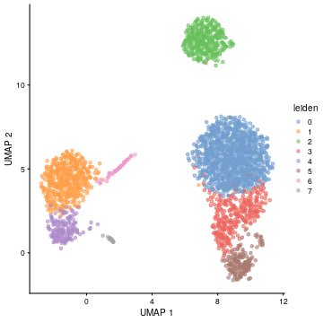
```

![](Session4_files/figure-html/plotUMAP-1.png)

---
## Time for an exercise!

Exercise on scRNAseq analysis with Bioconductor can be found [here](../../exercises/exercises/exercise4_exercise.html).

Answers can be found [here](../../exercises/answers/exercise4_answers.html).