20191009_tidyr.utf8

class: center, middle, inverse, title-slide

# Data wrangling with tidy
<html>
<div style="float:left">

</div>
<hr color='#EB811B' size=1px width=796px>
</html>
### Rockefeller University, Bioinformatics Resource Centre
### <a href="https://rockefelleruniversity.github.io/RU_tidyverse/" class="uri">https://rockefelleruniversity.github.io/RU_tidyverse/</a>

---

# Data wrangling with Tidy

Some problems we face when dealing with data regularly.

<ul>
 <li>Every dataset is different. Sometimes very different.</li>
 <li>There are many ways to do things. Everyone has their favorite syntax.</li>
</ul>

The issue:
Many fundamental data processing functions exist in Base R and beyond. Sometimes they can be inconsistent or unnecessarily complex. Especially when dealing with non-standard dataframes. The result is code that is confusing and doesn't flow i.e. nested functions

---
## What does it mean to be tidy?

Tidyverse is most importantly a philosophy for data analysis that more often then not makes wrangling data easier. The tidyverse community have built what they describe as an opinionated group of packages. These packages readily talk to one another.

<ul>
 <li>More efficient code</li>
 <li>Easier to remember syntax</li>
 <li>Easier to read syntax</li>
</ul>

You can read their <a href="https://cran.r-project.org/web/packages/tidyverse/vignettes/manifesto.html">manifesto</a> to get a better understanding of the tidy ethos. 
 
---
## What does it actually mean to be tidy?

<ul>
 <li>A defined vision for coding style in R 
 <li>A defined vision for data formats in R
 <li>A defined vision for package design in R
 <li>Unified set of community pushing in a cohesive direction
 <li>Critical mass of people to influence the way the whole R community evolves
</ul>

---
## What are the main tidy tools?

<ul>
 <li>ggplot2 – making pretty graphs 
 <li>readr – reading data into R 
 <li>dplyr – manipulating data 
 <li>tibble - working with tibbles 
 <li>tidyr – miscellaneous tools for tidying data
 <li>purrr - iterating over data 
 <li>stringr – working with strings 
 <li>forcats - working with factors 
</ul>

Other tools have now been made for the tidy community. This community also overlaps with bioconductor. But the packages above are the linchpins that hold it together.

---
## What we won't be doing today

We already have a course online for plotting, including ggplot.

https://rockefelleruniversity.github.io/Plotting_In_R/

---
# Lets get tidy!
First step lets load in the data we are using today

```r
load(file='dataset/my_tidy.Rdata')
```

---
## Are all data frames equal?

```r
head(df1)
```

```
## # A tibble: 6 x 5
## salmon_id common_name age_classbylength length_mm IGF1_ng_ml
## <dbl> <chr> <chr> <dbl> <dbl>
## 1 35032 Chinook salmon yearling 147 41.3
## 2 35035 Sockeye salmon juvenile 121 NA 
## 3 35036 Sockeye salmon juvenile 112 NA 
## 4 35037 Steelhead juvenile 220 42.7
## 5 35038 Steelhead juvenile 152 NA 
## 6 35033 Chinook salmon mixed age juvenile 444 62.1
```

```r
head(df2)
```

```
## # A tibble: 6 x 5
## salmon_id common_name age_classbylength variable value
## <dbl> <chr> <chr> <fct> <dbl>
## 1 35032 Chinook salmon yearling length_mm 147 
## 2 35032 Chinook salmon yearling IGF1_ng_ml 41.3
## 3 35033 Chinook salmon mixed age juvenile length_mm 444 
## 4 35033 Chinook salmon mixed age juvenile IGF1_ng_ml 62.1
## 5 35034 Sockeye salmon juvenile length_mm 139 
## 6 35034 Sockeye salmon juvenile IGF1_ng_ml NA
```

---
## Are all data frames equal?

```r
head(df3a)
```

```
## # A tibble: 6 x 5
## salmon_id common_name age_classbylength variable value
## <dbl> <chr> <chr> <fct> <dbl>
## 1 35032 Chinook salmon yearling length_mm 147
## 2 35033 Chinook salmon mixed age juvenile length_mm 444
## 3 35034 Sockeye salmon juvenile length_mm 139
## 4 35035 Sockeye salmon juvenile length_mm 121
## 5 35036 Sockeye salmon juvenile length_mm 112
## 6 35037 Steelhead juvenile length_mm 220
```

```r
head(df3b)
```

```
## # A tibble: 6 x 5
## salmon_id common_name age_classbylength variable value
## <dbl> <chr> <chr> <fct> <dbl>
## 1 35032 Chinook salmon yearling IGF1_ng_ml 41.3
## 2 35033 Chinook salmon mixed age juvenile IGF1_ng_ml 62.1
## 3 35034 Sockeye salmon juvenile IGF1_ng_ml NA 
## 4 35035 Sockeye salmon juvenile IGF1_ng_ml NA 
## 5 35036 Sockeye salmon juvenile IGF1_ng_ml NA 
## 6 35037 Steelhead juvenile IGF1_ng_ml 42.7
```

---
## What is a tidy dataset?

A tidy dataset is a data frame (or table) for which the following are true:

* Each variable has its own column
* Each observation has its own row
* Each value has its own cell

***Which of our dataframes is tidy?***
--
&nbsp;
Our first dataframe is tidy

---
## Why bother?

Consistent dataframe layouts help to ensure that all values are present and that relationships between data points are clear.

R is a vectorized programming language. R builds data frames from vectors, and R works best when its operation are vectorized. Tidy data utilizes of both of these aspects of R.

=> Precise and Fast

---
## Lets load in the tidyverse

```r
library(tidyverse)
```

```
## ── Attaching packages ─────────────────────────────────────────────────────────── tidyverse 1.3.0 ──
```

```
## ✔ ggplot2 3.2.1     ✔ purrr   0.3.3
## ✔ tibble  2.1.3     ✔ dplyr   0.8.3
## ✔ tidyr   1.0.0     ✔ stringr 1.4.0
## ✔ readr   1.3.1     ✔ forcats 0.4.0
```

```
## ── Conflicts ────────────────────────────────────────────────────────────── tidyverse_conflicts() ──
## ✖ dplyr::collapse()   masks IRanges::collapse()
## ✖ dplyr::combine()    masks Biobase::combine(), BiocGenerics::combine()
## ✖ dplyr::desc()       masks IRanges::desc()
## ✖ tidyr::expand()     masks S4Vectors::expand()
## ✖ dplyr::filter()     masks stats::filter()
## ✖ dplyr::first()      masks S4Vectors::first()
## ✖ dplyr::lag()        masks stats::lag()
## ✖ ggplot2::Position() masks BiocGenerics::Position(), base::Position()
## ✖ purrr::reduce()     masks GenomicRanges::reduce(), IRanges::reduce()
## ✖ dplyr::rename()     masks S4Vectors::rename()
## ✖ dplyr::select()     masks AnnotationDbi::select()
## ✖ dplyr::slice()      masks IRanges::slice()
```

---
# dplyr
This package contains a variety of tools to access and manipulate dataframes.

They have a common rationale:

![dplyr](./imgs/dplyr.png)

---
## dplyr::select - (pt1)
**Select** allows you to make a vector from a specific variable

```r
# Select one variable (common_name)
select(df1, common_name)
```

```
## # A tibble: 97 x 1
## common_name 
## <chr> 
## 1 Chinook salmon
## 2 Sockeye salmon
## 3 Sockeye salmon
## 4 Steelhead 
## 5 Steelhead 
## 6 Chinook salmon
## 7 Sockeye salmon
## 8 Steelhead 
## 9 Steelhead 
## 10 Steelhead 
## # … with 87 more rows
```

---
## dplyr::select - (pt2)
**Select** allows you to make a dataframe from several variables

```r
# Select two variables (age_classbylength and common_name)
select(df1, age_classbylength, common_name)
```

```
## # A tibble: 97 x 2
## age_classbylength common_name 
## <chr> <chr> 
## 1 yearling Chinook salmon
## 2 juvenile Sockeye salmon
## 3 juvenile Sockeye salmon
## 4 juvenile Steelhead 
## 5 juvenile Steelhead 
## 6 mixed age juvenile Chinook salmon
## 7 juvenile Sockeye salmon
## 8 juvenile Steelhead 
## 9 juvenile Steelhead 
## 10 juvenile Steelhead 
## # … with 87 more rows
```

---
## dplyr::select - (pt3)
**Select** allows you to make a dataframe excluding a variable

```r
# Select all but one variable (length_mm)
select(df1,-length_mm)
```

```
## # A tibble: 97 x 4
## salmon_id common_name age_classbylength IGF1_ng_ml
## <dbl> <chr> <chr> <dbl>
## 1 35032 Chinook salmon yearling 41.3
## 2 35035 Sockeye salmon juvenile NA 
## 3 35036 Sockeye salmon juvenile NA 
## 4 35037 Steelhead juvenile 42.7
## 5 35038 Steelhead juvenile NA 
## 6 35033 Chinook salmon mixed age juvenile 62.1
## 7 35034 Sockeye salmon juvenile NA 
## 8 35048 Steelhead juvenile 24.2
## 9 35049 Steelhead juvenile NA 
## 10 35050 Steelhead juvenile 63.5
## # … with 87 more rows
```

---
## dplyr::select - (pt4)
**Select** allows you to make a dataframe from a range of variables

```r
# Select all a range of contiguous varibles (common_name:length_mm)
select(df1, common_name:length_mm)
```

```
## # A tibble: 97 x 3
## common_name age_classbylength length_mm
## <chr> <chr> <dbl>
## 1 Chinook salmon yearling 147
## 2 Sockeye salmon juvenile 121
## 3 Sockeye salmon juvenile 112
## 4 Steelhead juvenile 220
## 5 Steelhead juvenile 152
## 6 Chinook salmon mixed age juvenile 444
## 7 Sockeye salmon juvenile 139
## 8 Steelhead juvenile 288
## 9 Steelhead juvenile 190
## 10 Steelhead juvenile 283
## # … with 87 more rows
```

---
## dplyr::filter - (pt1)
__Filter__ allows you to access observations based on a criteria

```r
# Filter all observation where the variable common_name is Sockeye salmon
filter(df1, common_name == 'Sockeye salmon')
```

```
## # A tibble: 11 x 5
## salmon_id common_name age_classbylength length_mm IGF1_ng_ml
## <dbl> <chr> <chr> <dbl> <dbl>
## 1 35035 Sockeye salmon juvenile 121 NA
## 2 35036 Sockeye salmon juvenile 112 NA
## 3 35034 Sockeye salmon juvenile 139 NA
## 4 35144 Sockeye salmon juvenile 140 NA
## 5 35147 Sockeye salmon juvenile 115 NA
## 6 35096 Sockeye salmon juvenile 115 NA
## 7 35097 Sockeye salmon juvenile 110 NA
## 8 35098 Sockeye salmon juvenile 112 NA
## 9 35099 Sockeye salmon juvenile 111 NA
## 10 35100 Sockeye salmon juvenile 118 NA
## 11 35119 Sockeye salmon juvenile 122 NA
```

---
## dplyr::filter - (pt2)
__Filter__ allows you to access observations based on several criteria

```r
# Filter all observations where the variable common_name is either Sockeye salmon or Chinook Salmon
filter(df1, common_name %in% c('Sockeye salmon', 'Chinook salmon'))
```

```
## # A tibble: 57 x 5
## salmon_id common_name age_classbylength length_mm IGF1_ng_ml
## <dbl> <chr> <chr> <dbl> <dbl>
## 1 35032 Chinook salmon yearling 147 41.3
## 2 35035 Sockeye salmon juvenile 121 NA 
## 3 35036 Sockeye salmon juvenile 112 NA 
## 4 35033 Chinook salmon mixed age juvenile 444 62.1
## 5 35034 Sockeye salmon juvenile 139 NA 
## 6 35142 Chinook salmon yearling 149 66.5
## 7 35143 Chinook salmon yearling 204 80.9
## 8 35144 Sockeye salmon juvenile 140 NA 
## 9 35145 Chinook salmon yearling 130 23.4
## 10 35146 Chinook salmon mixed age juvenile 422 101. 
## # … with 47 more rows
```

---
## dplyr::filter - (pt3)
__Filter__ allows you to access observations based on specific strings

```r
# Filter all observations where the variable common_name ends with 'salmon'. To do this we use stringr function str_ends recognise strings that end with 'salmon'.
filter(df1, str_ends(common_name, 'salmon'))
```

```
## # A tibble: 59 x 5
## salmon_id common_name age_classbylength length_mm IGF1_ng_ml
## <dbl> <chr> <chr> <dbl> <dbl>
## 1 35032 Chinook salmon yearling 147 41.3
## 2 35035 Sockeye salmon juvenile 121 NA 
## 3 35036 Sockeye salmon juvenile 112 NA 
## 4 35033 Chinook salmon mixed age juvenile 444 62.1
## 5 35034 Sockeye salmon juvenile 139 NA 
## 6 35142 Chinook salmon yearling 149 66.5
## 7 35143 Chinook salmon yearling 204 80.9
## 8 35144 Sockeye salmon juvenile 140 NA 
## 9 35145 Chinook salmon yearling 130 23.4
## 10 35146 Chinook salmon mixed age juvenile 422 101. 
## # … with 49 more rows
```

---
## dplyr::filter - (pt4)
__Filter__ allows you to access observations based on operators

```r
# Filter all observations where the variable length_mm is greater than 200 or less than 120
filter(df1, length_mm > 200 | length_mm < 120)
```

```
## # A tibble: 36 x 5
## salmon_id common_name age_classbylength length_mm IGF1_ng_ml
## <dbl> <chr> <chr> <dbl> <dbl>
## 1 35036 Sockeye salmon juvenile 112 NA 
## 2 35037 Steelhead juvenile 220 42.7
## 3 35033 Chinook salmon mixed age juvenile 444 62.1
## 4 35048 Steelhead juvenile 288 24.2
## 5 35050 Steelhead juvenile 283 63.5
## 6 35051 Steelhead juvenile 279 61.2
## 7 35052 Steelhead juvenile 235 30.6
## 8 35053 Steelhead juvenile 230 49.4
## 9 35056 Steelhead juvenile 208 57.4
## 10 35057 Steelhead juvenile 240 20.2
## # … with 26 more rows
```

---
## CHALLENGE: Time for an exercise!

Exercise on dplyr's select and filter can be found [here](http://rockefelleruniversity.github.io/RU_tidyverse/tidyR/exercises/EX1_RU_tidyverse_dplyr_select_and_filter.html)

---
### Answers to exercise.

Answers can be found [here](http://rockefelleruniversity.github.io/RU_tidyverse/tidyR/answers/EX1_ANSWERS_RU_tidyverse_dplyr_select_and_filter.html)

R code for solutions can be found [here](http://rockefelleruniversity.github.io/RU_tidyverse/tidyR/answers/EX1_ANSWERS_RU_tidyverse_dplyr_select_and_filter.R)

---
## dplyr::arrange - (pt1)
_Arrange_ sorts the dataframe based on a specific variable

```r
# Arrange the data based on the variable length_mm
arrange(df1, length_mm)
```

```
## # A tibble: 97 x 5
## salmon_id common_name age_classbylength length_mm IGF1_ng_ml
## <dbl> <chr> <chr> <dbl> <dbl>
## 1 35095 Chinook salmon subyearling 90 NA
## 2 35097 Sockeye salmon juvenile 110 NA
## 3 35099 Sockeye salmon juvenile 111 NA
## 4 35036 Sockeye salmon juvenile 112 NA
## 5 35098 Sockeye salmon juvenile 112 NA
## 6 35147 Sockeye salmon juvenile 115 NA
## 7 35096 Sockeye salmon juvenile 115 NA
## 8 35100 Sockeye salmon juvenile 118 NA
## 9 35035 Sockeye salmon juvenile 121 NA
## 10 35119 Sockeye salmon juvenile 122 NA
## # … with 87 more rows
```
---
## dplyr::arrange - (pt2)
_Arrange_ sorts the dataframe based on specific variables

```r
# Arrange the data first based on the variable common_name, 
# then secondly based on length_mm in a descending order.
arrange(df1, common_name, desc(length_mm))
```

```
## # A tibble: 97 x 5
## salmon_id common_name age_classbylength length_mm IGF1_ng_ml
## <dbl> <chr> <chr> <dbl> <dbl>
## 1 35033 Chinook salmon mixed age juvenile 444 62.1 
## 2 35146 Chinook salmon mixed age juvenile 422 101. 
## 3 35110 Chinook salmon mixed age juvenile 275 81.5 
## 4 35129 Chinook salmon yearling 225 72.7 
## 5 35103 Chinook salmon yearling 216 81.2 
## 6 35115 Chinook salmon yearling 215 53.5 
## 7 35112 Chinook salmon yearling 205 90.5 
## 8 35143 Chinook salmon yearling 204 80.9 
## 9 35079 Chinook salmon yearling 199 53.2 
## 10 35081 Chinook salmon yearling 196 5.56
## # … with 87 more rows
```

---
## dplyr::mutate - (pt1)
_Mutate_ creates a new variable based on some form of computation

```r
# A new variable is created based on the calculation of the
# z-score of the variable IGF1_ng_ml using scale()
mutate(df1, scale(IGF1_ng_ml))
```

```
## # A tibble: 97 x 6
## salmon_id common_name age_classbylength length_mm IGF1_ng_ml `scale(IGF1_ng_ml)`[,1]
## <dbl> <chr> <chr> <dbl> <dbl> <dbl>
## 1 35032 Chinook salmon yearling 147 41.3 -0.258
## 2 35035 Sockeye salmon juvenile 121 NA NA 
## 3 35036 Sockeye salmon juvenile 112 NA NA 
## 4 35037 Steelhead juvenile 220 42.7 -0.191
## 5 35038 Steelhead juvenile 152 NA NA 
## 6 35033 Chinook salmon mixed age juvenile 444 62.1 0.704
## 7 35034 Sockeye salmon juvenile 139 NA NA 
## 8 35048 Steelhead juvenile 288 24.2 -1.04 
## 9 35049 Steelhead juvenile 190 NA NA 
## 10 35050 Steelhead juvenile 283 63.5 0.766
## # … with 87 more rows
```
---
## dplyr::mutate - (pt2)
_Mutate_ creates a named variable based on some form of computation

```r
# A new variable is created called IGFngml_zscore, based on the 
# calculation of the z-score of the variable IGF1_ng_ml using scale()
mutate(df1, IGFngml_zscore = scale(IGF1_ng_ml))
```

```
## # A tibble: 97 x 6
## salmon_id common_name age_classbylength length_mm IGF1_ng_ml IGFngml_zscore[,1]
## <dbl> <chr> <chr> <dbl> <dbl> <dbl>
## 1 35032 Chinook salmon yearling 147 41.3 -0.258
## 2 35035 Sockeye salmon juvenile 121 NA NA 
## 3 35036 Sockeye salmon juvenile 112 NA NA 
## 4 35037 Steelhead juvenile 220 42.7 -0.191
## 5 35038 Steelhead juvenile 152 NA NA 
## 6 35033 Chinook salmon mixed age juvenile 444 62.1 0.704
## 7 35034 Sockeye salmon juvenile 139 NA NA 
## 8 35048 Steelhead juvenile 288 24.2 -1.04 
## 9 35049 Steelhead juvenile 190 NA NA 
## 10 35050 Steelhead juvenile 283 63.5 0.766
## # … with 87 more rows
```

---
## CHALLENGE: Time for an exercise!

Exercise on dplyr's arrange and mutate can be found [here](http://rockefelleruniversity.github.io/RU_tidyverse/tidyR/exercises/EX2_RU_tidyverse_dplyr_arrange_and_mutate.html)

---
### Answers to exercise.

Answers can be found [here](http://rockefelleruniversity.github.io/RU_tidyverse/tidyR/answers/EX2_ANSWERS_RU_tidyverse_dplyr_arrange_and_mutate.html)

R code for solutions can be found [here](http://rockefelleruniversity.github.io/RU_tidyverse/tidyR/answers/EX2_ANSWERS_RU_tidyverse_dplyr_arrange_and_mutate.R)

---
## dplyr::summarize - (pt1)
_Summarize_ applies aggregating or summary function to a group i.e. counting

```r
# First we define the common_name as a group. 
df1_byname <- group_by(df1, common_name)

# Summarise is used to count over the grouped common_names
summarise(df1_byname, count = n())
```

```
## # A tibble: 4 x 2
## common_name count
## <chr> <int>
## 1 Chinook salmon 46
## 2 Coho salmon 2
## 3 Sockeye salmon 11
## 4 Steelhead 38
```
---
## dplyr::summarize - (pt2)
_Summarize_ applies aggregating or summary function to a group i.e. means

```r
# Summarise is used to calculate mean IGF1_ng_ml over the
# grouped common_names
summarise(df1_byname, IGF1_ng_ml_ave = mean(IGF1_ng_ml, na.rm = T))
```

```
## # A tibble: 4 x 2
## common_name IGF1_ng_ml_ave
## <chr> <dbl>
## 1 Chinook salmon 46.8
## 2 Coho salmon 73.6
## 3 Sockeye salmon NaN 
## 4 Steelhead 46.1
```

---
## dplyr::group_by - (pt1)
_Grouping_ can also help filter within groups

```r
# Filter observations with the 2 smallest length_mm for each grouped common_names
filter(df1_byname, rank(length_mm) <= 2)
```

```
## # A tibble: 8 x 5
## # Groups: common_name [4]
## salmon_id common_name age_classbylength length_mm IGF1_ng_ml
## <dbl> <chr> <chr> <dbl> <dbl>
## 1 35038 Steelhead juvenile 152 NA 
## 2 35055 Steelhead juvenile 123 55.7
## 3 35145 Chinook salmon yearling 130 23.4
## 4 35085 Coho salmon yearling 140 NA 
## 5 35087 Coho salmon yearling 164 73.6
## 6 35095 Chinook salmon subyearling 90 NA 
## 7 35097 Sockeye salmon juvenile 110 NA 
## 8 35099 Sockeye salmon juvenile 111 NA
```
---
## dplyr::group_by - (pt2)
_Grouping_ can also help filter within groups

```r
# Filter observations with at least 5 for each grouped common_names
filter(df1_byname, n() > 5)
```

```
## # A tibble: 95 x 5
## # Groups: common_name [3]
## salmon_id common_name age_classbylength length_mm IGF1_ng_ml
## <dbl> <chr> <chr> <dbl> <dbl>
## 1 35032 Chinook salmon yearling 147 41.3
## 2 35035 Sockeye salmon juvenile 121 NA 
## 3 35036 Sockeye salmon juvenile 112 NA 
## 4 35037 Steelhead juvenile 220 42.7
## 5 35038 Steelhead juvenile 152 NA 
## 6 35033 Chinook salmon mixed age juvenile 444 62.1
## 7 35034 Sockeye salmon juvenile 139 NA 
## 8 35048 Steelhead juvenile 288 24.2
## 9 35049 Steelhead juvenile 190 NA 
## 10 35050 Steelhead juvenile 283 63.5
## # … with 85 more rows
```
---
## dplyr::group_by - (pt3)
_Grouping_ creates a new variable based on some form of computation within the group

```r
# A new variable is created using z-score within the grouped common_names
mutate(df1_byname, IGFngml_zscore = scale(IGF1_ng_ml))
```

```
## # A tibble: 97 x 6
## # Groups: common_name [4]
## salmon_id common_name age_classbylength length_mm IGF1_ng_ml IGFngml_zscore
## <dbl> <chr> <chr> <dbl> <dbl> <dbl>
## 1 35032 Chinook salmon yearling 147 41.3 -0.236
## 2 35035 Sockeye salmon juvenile 121 NA NA 
## 3 35036 Sockeye salmon juvenile 112 NA NA 
## 4 35037 Steelhead juvenile 220 42.7 -0.176
## 5 35038 Steelhead juvenile 152 NA NA 
## 6 35033 Chinook salmon mixed age juvenile 444 62.1 0.652
## 7 35034 Sockeye salmon juvenile 139 NA NA 
## 8 35048 Steelhead juvenile 288 24.2 -1.12 
## 9 35049 Steelhead juvenile 190 NA NA 
## 10 35050 Steelhead juvenile 283 63.5 0.890
## # … with 87 more rows
```

---
## CHALLENGE: Time for an exercise!

Exercise on dplyr's grouping and summarize can be found [here](http://rockefelleruniversity.github.io/RU_tidyverse/tidyR/exercises/EX3_RU_tidyverse_dplyr_group_and_summarize.html)

---
### Answers to exercise.

Answers can be found [here](http://rockefelleruniversity.github.io/RU_tidyverse/tidyR/answers/EX3_ANSWERS_RU_tidyverse_dplyr_group_and_summarize.html)

R code for solutions can be found [here](http://rockefelleruniversity.github.io/RU_tidyverse/tidyR/answers/EX3_ANSWERS_RU_tidyverse_dplyr_group_and_summarize.R)

---
# Piping to string functions together

Piping was allows you to pass the result from one expression directly into another.  
magrittR package developed the %>% pipe which is integral to the tidy way of formatting code

The pattern is similar but now follows a specific logical flow:

![dplyr](./imgs/dplyr_pipe.png)
---
## Piping vs. not piping

```r
# Without pipe
df1_byname <- group_by(df1, common_name)
summarise(df1_byname, IGF1_ng_ml_ave = mean(IGF1_ng_ml, na.rm=T))
```

```r
# With pipe
df1 %>% 
  group_by(common_name) %>% 
  summarise(IGF1_ng_ml_ave = mean(IGF1_ng_ml, na.rm=T))
```

---
## Linking functions with pipes - (pt1)

```r
# (1) Group by common_name
# (2) Filter to all those that have length bigger then 200
# (3) Summarise is used to calculate mean IGF1_ng_ml over the grouped 
# common_names for these larger fish

df1 %>%
  group_by(common_name) %>% 
  filter(length_mm > 200) %>% 
  summarise(IGF1_ng_ml_ave = mean(IGF1_ng_ml, na.rm = T))
```

```
## # A tibble: 2 x 2
## common_name IGF1_ng_ml_ave
## <chr> <dbl>
## 1 Chinook salmon 77.9
## 2 Steelhead 45.3
```
---
## Linking functions with pipes - (pt2)

```r
# (1) Create new variable that is discrete label depending on size of the fish
# (2) Group by common_name and size
# (3) Summarise is used to calculate mean IGF1_ng_ml over the grouped 
# common_names and sizes

df1 %>%
  mutate(size = if_else(length_mm > 200, 'big_fish', 'small_fish')) %>% 
  group_by(common_name, size) %>% 
  summarise(IGF1_ng_ml_ave = mean(IGF1_ng_ml, na.rm = T))
```

```
## # A tibble: 6 x 3
## # Groups: common_name [4]
## common_name size IGF1_ng_ml_ave
## <chr> <chr> <dbl>
## 1 Chinook salmon big_fish 77.9
## 2 Chinook salmon small_fish 39.5
## 3 Coho salmon small_fish 73.6
## 4 Sockeye salmon small_fish NaN 
## 5 Steelhead big_fish 45.3
## 6 Steelhead small_fish 47.3
```
---
## Linking functions with pipes - (pt3)

df1 %>%
  mutate(size = if_else(length_mm > 200, 'big_fish', 'small_fish')) %>% 
  group_by(common_name, size) %>% 
  summarise(IGF1_ng_ml_ave = mean(IGF1_ng_ml, na.rm = T)) %>%
  filter(common_name != 'Coho salmon')  %>%
  filter(common_name !='Sockeye salmon')
```

```
## # A tibble: 4 x 3
## # Groups: common_name [2]
## common_name size IGF1_ng_ml_ave
## <chr> <chr> <dbl>
## 1 Chinook salmon big_fish 77.9
## 2 Chinook salmon small_fish 39.5
## 3 Steelhead big_fish 45.3
## 4 Steelhead small_fish 47.3
```

---
## You can pipe straight to plots - (pt1)

```r
p <- df1 %>% mutate(size=if_else(length_mm>200, 'big_fish', 'small_fish')) %>% 
 group_by(common_name, size) %>% 
 summarize(IGF1_ng_ml_ave=mean(IGF1_ng_ml, na.rm=T)) %>% 
 filter(common_name != 'Coho salmon') %>% 
 filter(common_name != 'Sockeye salmon') %>% 
 ggplot(aes(x = common_name, y = IGF1_ng_ml_ave, group = size, fill = size)) +
 geom_bar(stat = "identity", position = "dodge") + 
 theme(axis.text.x = element_text(angle = 90)) +
 scale_fill_brewer(palette = "Paired")
```
---
## You can pipe straight to plots - (pt2)

```r
p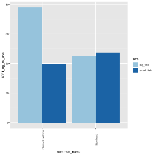
```

![](20191009_tidyr_files/figure-html/unnamed-chunk-29-1.png)

---
## CHALLENGE: Time for an exercise!

Exercise on piping can be found [here](http://rockefelleruniversity.github.io/RU_tidyverse/tidyR/exercises/EX4_RU_tidyverse_pipes.html)

---
### Answers to exercise.

Answers can be found [here](http://rockefelleruniversity.github.io/RU_tidyverse/tidyR/answers/EX4_ANSWERS_RU_tidyverse_pipes.html)

R code for solutions can be found [here](http://rockefelleruniversity.github.io/RU_tidyverse/tidyR/answers/EX4_ANSWERS_RU_tidyverse_pipes.R)

---
# readr: Reading data into R
So we blasted through what being tidy can give you. 
Now lets start from the beginning and tidy some data. First step is to read in data.

readr:

* read_csv(): comma separated (CSV) files  
* read_tsv(): tab separated files  
* read_delim(): general delimited files  
* read_fwf(): fixed width files  
* read_table(): tabular files where columns are separated by white-space  
* read_log(): web log files

---
## Reading in with base

```r
untidy_counts_base <- read.csv("dataset/hemato_rnaseq_counts.csv")
# Base will print out everything
untidy_counts_base
```

```
##     ENTREZ CD34_1 ORTHO_1 CD34_2 ORTHO_2
## 1      350    204       0    103       0
## 2      351  15586     479  10476      39
## 3      353    842     355   1188      86
## 4      354      0       0      0       0
## 5      355    123     291    139      16
## 6      356      1       1      0       0
## 7      357    380       3    177       0
## 8      358    572    2225    597    4051
## 9      359      0      12      1       0
## 10     360    320     502     46    1114
## 11     361      0       1      0       0
## 12     362      3       1     15       0
## 13     363     14       6      4       1
## 14     364      7       0      1       0
## 15     366      6       0      1       0
## 16     367     42       0     51       1
## 17     368     28       0     24       0
## 18     369   1204    1034    833     478
## 19     372   2829    1864   2741     771
## 20     373    179     728    148     795
## 21     374     76       5    138       2
## 22     375   4428    6697   4970    4328
## 23     377   3170     314   2576      11
## 24     378   1839    4845   1767    2975
## 25     379    178       1    181       0
## 26     381   1617     574   1159     339
## 27     382   2874    2265   1746    1668
## 28     383     63    1632     40     721
## 29     384    148   10977    118      94
## 30     387   8899    2457   7405    1228
## 31     388  12598     171   5090      70
## 32     389   2709     193   2313       5
## 33     390   1004       0    395       0
## 34     391   1038     577   1176     164
## 35     392   1527     304    786      71
## 36     393   2949     138   1540       3
## 37     394   1525     464   1062     134
## 38     395    348      67    123       0
## 39     396   6503     702   4723     169
## 40     397  12997     410  11265      38
## 41     398      0       0      0       0
## 42     399    223      11    422       2
## 43     400   1188     147    806      56
## 44     401      0       0      0       0
## 45     402    504     218    496      80
## 46     403    289      25    166       4
## 47     405   1481     824   1004     812
## 48     406    295     175     87      35
## 49     407      4       1      2       1
## 50     408   2451     111   1523       6
## 51     409   2480    1819   1356     226
## 52     410    433     197    215      77
## 53     411    829     217    441     131
## 54     412    312      45    138      17
## 55     414    516      15    396       9
## 56     415     20       0     13       0
## 57     416      2       1      4       0
## 58     417      0       0      0       0
## 59     419      6       5      2       7
## 60     420    141    1136     94    1217
## 61     421    213     255     93     208
## 62     427   4699   11889   1729     926
## 63     429      0       0      2       0
## 64     430     34      13     22       0
## 65     432     63       0     55       1
## 66     433     38       0     26       0
## 67     434      1       1      2       0
## 68     435    408     151    284      34
## 69     440    157    2520    111     535
## 70     443      5       0      4       0
## 71     444   1583     151    747      14
## 72     445    116      15     90       1
## 73     460     34       0     68       0
## 74     462     70       0     31       1
## 75     463   1244     118    492      71
## 76     466    538     480    393     218
## 77     467   2506     402   2130      18
## 78     468   7991    6132   5307    1883
## 79     471   1272     771   1392      53
## 80     472   1389     628    739     138
## 81     473   4173     783   1901     776
## 82     474      0       0      0       0
## 83     475    284      83    467      34
## 84     476   4952    3453   4202    1416
## 85     477     13       3     26       2
## 86     478     78     121     67       0
## 87     479     17       0      4       0
## 88     480      9       5     11       1
## 89     481   1937      18   1017      34
## 90     482    157    1392     75    1660
## 91     483   1075    1454   1789    1141
## 92     486     47       0     18       0
## 93     487     29      33     19       3
## 94     488   4529    1118   2925     269
## 95     489   3465     153   3188       8
## 96     490   1610    1263    913     665
## 97     491     12       1      4       0
## 98     492      4       0      6       0
## 99     493   5011    3585   3053     743
## 100    495      0       0      0       0
```
---
## Reading in with readr - (pt1)

```r
# readr gives you a tibble. 
read_csv("dataset/hemato_rnaseq_counts.csv")
```

```
## Parsed with column specification:
## cols(
##   ENTREZ = col_double(),
##   CD34_1 = col_double(),
##   ORTHO_1 = col_double(),
##   CD34_2 = col_double(),
##   ORTHO_2 = col_double()
## )
```

```
## # A tibble: 100 x 5
## ENTREZ CD34_1 ORTHO_1 CD34_2 ORTHO_2
## <dbl> <dbl> <dbl> <dbl> <dbl>
## 1 350 204 0 103 0
## 2 351 15586 479 10476 39
## 3 353 842 355 1188 86
## 4 354 0 0 0 0
## 5 355 123 291 139 16
## 6 356 1 1 0 0
## 7 357 380 3 177 0
## 8 358 572 2225 597 4051
## 9 359 0 12 1 0
## 10 360 320 502 46 1114
## # … with 90 more rows
```
---
## Reading in with readr - (pt2)

```r
# Tibbles carry and display extra information. 
# While reading in it is easy to specify data type. 
untidy_counts <- read_csv("dataset/hemato_rnaseq_counts.csv", col_types = cols(
 ENTREZ = col_character(),
 CD34_1 = col_integer(),
 ORTHO_1 = col_integer(),
 CD34_2 = col_integer(),
 ORTHO_2 = col_integer()
 ))
untidy_counts
```

```
## # A tibble: 100 x 5
## ENTREZ CD34_1 ORTHO_1 CD34_2 ORTHO_2
## <chr> <int> <int> <int> <int>
## 1 350 204 0 103 0
## 2 351 15586 479 10476 39
## 3 353 842 355 1188 86
## 4 354 0 0 0 0
## 5 355 123 291 139 16
## 6 356 1 1 0 0
## 7 357 380 3 177 0
## 8 358 572 2225 597 4051
## 9 359 0 12 1 0
## 10 360 320 502 46 1114
## # … with 90 more rows
```

---
## Subsetting to make tibbles - (pt1)

```r
# Can use the same way as base to interact with the 
# tibble dataframe - columns
untidy_counts[,1]
```

```
## # A tibble: 100 x 1
## ENTREZ
## <chr> 
## 1 350 
## 2 351 
## 3 353 
## 4 354 
## 5 355 
## 6 356 
## 7 357 
## 8 358 
## 9 359 
## 10 360 
## # … with 90 more rows
```
---
## Subsetting to make tibbles - (pt2)

```r
# Can use the same way as base to interact with the
# tibble dataframe - rows
untidy_counts[1,]
```

```
## # A tibble: 1 x 5
## ENTREZ CD34_1 ORTHO_1 CD34_2 ORTHO_2
## <chr> <int> <int> <int> <int>
## 1 350 204 0 103 0
```
---
## Subsetting to make tibbles - (pt3)

```r
# Can also not specify which dimension you pull from. 
# This will default to grabbing the column
untidy_counts[1]
```

```
## # A tibble: 100 x 1
## ENTREZ
## <chr> 
## 1 350 
## 2 351 
## 3 353 
## 4 354 
## 5 355 
## 6 356 
## 7 357 
## 8 358 
## 9 359 
## 10 360 
## # … with 90 more rows
```
---
## Subsetting to make vectors - (pt1)

```r
# All the prior outputs have been outputting another tibble. 
# If double brackets are used a vector is returned 
untidy_counts[[1]]
```

```
##   [1] "350" "351" "353" "354" "355" "356" "357" "358" "359" "360" "361" "362" "363" "364" "366"
##  [16] "367" "368" "369" "372" "373" "374" "375" "377" "378" "379" "381" "382" "383" "384" "387"
##  [31] "388" "389" "390" "391" "392" "393" "394" "395" "396" "397" "398" "399" "400" "401" "402"
##  [46] "403" "405" "406" "407" "408" "409" "410" "411" "412" "414" "415" "416" "417" "419" "420"
##  [61] "421" "427" "429" "430" "432" "433" "434" "435" "440" "443" "444" "445" "460" "462" "463"
##  [76] "466" "467" "468" "471" "472" "473" "474" "475" "476" "477" "478" "479" "480" "481" "482"
##  [91] "483" "486" "487" "488" "489" "490" "491" "492" "493" "495"
```
---
## Subsetting to make vectors - (pt2)

```r
# This is also the case if you use the dollar and colname 
# to access a column
untidy_counts$ENTREZ
```

---
## CHALLENGE: Time for an exercise!

Exercise on readr can be found [here](http://rockefelleruniversity.github.io/RU_tidyverse/tidyR/exercises/EX5_RU_tidyverse_readr.html)

---
### Answers to exercise.

Answers can be found [here](http://rockefelleruniversity.github.io/RU_tidyverse/tidyR/answers/EX5_ANSWERS_RU_tidyverse_readr.html)

R code for solutions can be found [here](http://rockefelleruniversity.github.io/RU_tidyverse/tidyR/answers/EX5_ANSWERS_RU_tidyverse_readr.R)

---
## Tibbles: Converting to tibble - (pt1)

```r
# Can convert base dataframes into tibbles
as_tibble(untidy_counts_base)
```

```
## # A tibble: 100 x 5
## ENTREZ CD34_1 ORTHO_1 CD34_2 ORTHO_2
## <int> <int> <int> <int> <int>
## 1 350 204 0 103 0
## 2 351 15586 479 10476 39
## 3 353 842 355 1188 86
## 4 354 0 0 0 0
## 5 355 123 291 139 16
## 6 356 1 1 0 0
## 7 357 380 3 177 0
## 8 358 572 2225 597 4051
## 9 359 0 12 1 0
## 10 360 320 502 46 1114
## # … with 90 more rows
```
---
## Tibbles: Converting to tibble - (pt2)

```r
# Once it is a tibble it is straight forward to modify the datatype
untidy_counts_base <- as_tibble(untidy_counts_base) %>%
 mutate_at(vars(ENTREZ), as.character)
untidy_counts_base
```

```r
# Some tools are not tibble friendly. Calling as.data.frame is 
# sufficient to convert it back to a base data frame
as.data.frame(untidy_counts_base) %>% head(n=12)
```

---
## Tibbles: Make your own - (pt1)
__We will make our own tibble now from scratch, using some metadata that will be useful later__

```r
# Lets load in some packages
library(org.Hs.eg.db)
library(TxDb.Hsapiens.UCSC.hg19.knownGene)

# Lets use the ENTREZ ID as a key
keys <- untidy_counts$ENTREZ

# We can use the ENTREZ ID to look up Gene Symbol
symbols <- select(org.Hs.eg.db, keys = keys,columns = "SYMBOL", keytype = "ENTREZID")

# We can use the ENTREZ ID to look up the chormosome the gene resides on
chrs <- select(TxDb.Hsapiens.UCSC.hg19.knownGene, keys = keys, columns = "TXCHROM", keytype = "GENEID")

# We can use the ENTREZ ID to get a list of genes with grange of their exons
geneExons <- exonsBy(TxDb.Hsapiens.UCSC.hg19.knownGene,by = "gene")[keys]
```

---
## Tibbles: Make your own - (pt2)

```r
# We will then use an apply to get the transcript length from each gene in the 
# list. The transcript length is calculated by first flattening overlapping 
# exons with reduce(), then calculating the length of each exon with width(), 
# then summing upthe total exon length to get our transcript length. 
txsLength <- sapply(geneExons, function(x){ x %>%
 GenomicRanges::reduce() %>%
 width() %>%
 sum() })

# Finally we have all this metadata. Lets put it together into a tibble. 
counts_metadata <- tibble(ID = symbols$ENTREZID, SYMBOL = symbols$SYMBOL, CHR = chrs$TXCHROM, LENGTH = txsLength)
```

---
## Tibbles: Make your own - (pt3)

```r
counts_metadata
```

```
## # A tibble: 100 x 4
## ID SYMBOL CHR LENGTH
## <chr> <chr> <chr> <int>
## 1 350 APOH chr17 1201
## 2 351 APP chr21 4480
## 3 353 APRT chr16 807
## 4 354 KLK3 chr19 1906
## 5 355 FAS chr10 6691
## 6 356 FASLG chr1 1859
## 7 357 SHROOM2 chrX 8206
## 8 358 AQP1 chr7 3786
## 9 359 AQP2 chr12 4179
## 10 360 AQP3 chr9 2950
## # … with 90 more rows
```

---
# Tidying data up

What is wrong with the count dataframe from a tidy viewpoint?

_Remember_. These are the rules:

* Each variable has its own column
* Each observation has its own row
* Each value has its own cell

```r
untidy_counts
```

---
## Tidying data up

What is wrong with the count dataframe from a tidy viewpoint?

_Remember_, these are the rules:

* Each variable has its own column
* Each observation has its own row
* Each value has its own cell

__A single variable with multiple columns__

```r
untidy_counts
```

---
## Reshape data with gather and spread

When all the content is in the data frame, but it is in the wrong orientation, tidyr has some tools to move the data around quickly and easily:

__gather and spread__

---
## tidyr::gather 
Gather allows you to collapse single varibles that are spread over multiple columns

```r
# New columns Sample and Counts are created from whole dataframe
tidier_counts <- gather(untidy_counts, key="Sample", value="counts", -ENTREZ)
tidier_counts
```

```
## # A tibble: 400 x 3
## ENTREZ Sample counts
## <chr> <chr> <int>
## 1 350 CD34_1 204
## 2 351 CD34_1 15586
## 3 353 CD34_1 842
## 4 354 CD34_1 0
## 5 355 CD34_1 123
## 6 356 CD34_1 1
## 7 357 CD34_1 380
## 8 358 CD34_1 572
## 9 359 CD34_1 0
## 10 360 CD34_1 320
## # … with 390 more rows
```
---
## tidyr::spread
Spread allows you to spread single variables over multiple columns

```r
spread(tidier_counts, key="Sample", value="counts")
```

```
## # A tibble: 100 x 5
## ENTREZ CD34_1 CD34_2 ORTHO_1 ORTHO_2
## <chr> <int> <int> <int> <int>
## 1 350 204 103 0 0
## 2 351 15586 10476 479 39
## 3 353 842 1188 355 86
## 4 354 0 0 0 0
## 5 355 123 139 291 16
## 6 356 1 0 1 0
## 7 357 380 177 3 0
## 8 358 572 597 2225 4051
## 9 359 0 1 12 0
## 10 360 320 46 502 1114
## # … with 90 more rows
```
---
## tidyr::pivot_longer/pivot_wider
Gather and spread are being retired. They are being replaced with pivot_tools. 
There is slightly different nomencalture, but they pretty much do the same thing.

```r
#
pivot_longer(untidy_counts,names_to = "Sample", values_to = "counts", cols = c(-ENTREZ))
gather(untidy_counts, key=Sample, value=counts, -ENTREZ)
# 
pivot_wider(tidier_counts, names_from = c(Sample), values_from = counts)
spread(tidier_counts, key=Sample, value=counts)
```

---
## CHALLENGE: Time for an exercise!

Exercise on tidying can be found [here](http://rockefelleruniversity.github.io/RU_tidyverse/tidyR/exercises/EX6_RU_tidyverse_tidying.html)

---
### Answers to exercise.

Answers can be found [here](http://rockefelleruniversity.github.io/RU_tidyverse/tidyR/answers/EX6_ANSWERS_RU_tidyverse_tidying.html)

R code for solutions can be found [here](http://rockefelleruniversity.github.io/RU_tidyverse/tidyR/answers/EX6_ANSWERS_RU_tidyverse_tidying.R)

---
## What is next to tidy?

_Remember_, these are the rules:

* Each variable has its own column
* Each observation has its own row
* Each value has its own cell

```r
tidier_counts
```

---
## What is next to tidy?

_Remember_, these are the rules:

* Each variable has its own column
* Each observation has its own row
* Each value has its own cell

__Multiple variables in a single column__

```r
tidier_counts
```

---
## Splitting and combining varaibles

When there are several variables crammed into a single column, tidyr can be used to split single values into several:

__separate__

---
## tidyr::separate - (pt1)

```r
# Separate allows you to break a strings in a variable by a separator.
# In this case the cell type and replicate number are broken by underscore
tidier_counts <- separate(tidier_counts, Sample, sep = "_", into=c("CellType","Rep"), remove=TRUE)
tidier_counts
```

```
## # A tibble: 400 x 4
## ENTREZ CellType Rep counts
## <chr> <chr> <chr> <int>
## 1 350 CD34 1 204
## 2 351 CD34 1 15586
## 3 353 CD34 1 842
## 4 354 CD34 1 0
## 5 355 CD34 1 123
## 6 356 CD34 1 1
## 7 357 CD34 1 380
## 8 358 CD34 1 572
## 9 359 CD34 1 0
## 10 360 CD34 1 320
## # … with 390 more rows
```
---
## tidyr::unite

```r
# Unite can go the other way. This can sometime be useful i.e. if you want a specific sample ID
unite(tidier_counts, Sample, CellType, Rep, remove=FALSE)
```

```
## # A tibble: 400 x 5
## ENTREZ Sample CellType Rep counts
## <chr> <chr> <chr> <chr> <int>
## 1 350 CD34_1 CD34 1 204
## 2 351 CD34_1 CD34 1 15586
## 3 353 CD34_1 CD34 1 842
## 4 354 CD34_1 CD34 1 0
## 5 355 CD34_1 CD34 1 123
## 6 356 CD34_1 CD34 1 1
## 7 357 CD34_1 CD34 1 380
## 8 358 CD34_1 CD34 1 572
## 9 359 CD34_1 CD34 1 0
## 10 360 CD34_1 CD34 1 320
## # … with 390 more rows
```
---
## tidyr::separate - (pt2)

```r
# Remember you can always pipe everything together into a single expression
tidy_counts <- untidy_counts %>% 
 gather(key=Sample, value=counts, -ENTREZ) %>% 
 separate(Sample, sep = "_", into = c("CellType","Rep"), remove=FALSE)
tidy_counts
```

---
# Joining
Data frames can be joined on a shared variable _a.k.a._ a key. We want this key to be unique i.e. ENTREZ ID. 
---
## dplyr::inner_join - Merging dataframes

```r
tidy_counts
```

```r
counts_metadata
```

```r
inner_join(tidy_counts, counts_metadata, by = c("ENTREZ" = "ID"))
```

```
## # A tibble: 400 x 8
## ENTREZ Sample CellType Rep counts SYMBOL CHR LENGTH
## <chr> <chr> <chr> <chr> <int> <chr> <chr> <int>
## 1 350 CD34_1 CD34 1 204 APOH chr17 1201
## 2 351 CD34_1 CD34 1 15586 APP chr21 4480
## 3 353 CD34_1 CD34 1 842 APRT chr16 807
## 4 354 CD34_1 CD34 1 0 KLK3 chr19 1906
## 5 355 CD34_1 CD34 1 123 FAS chr10 6691
## 6 356 CD34_1 CD34 1 1 FASLG chr1 1859
## 7 357 CD34_1 CD34 1 380 SHROOM2 chrX 8206
## 8 358 CD34_1 CD34 1 572 AQP1 chr7 3786
## 9 359 CD34_1 CD34 1 0 AQP2 chr12 4179
## 10 360 CD34_1 CD34 1 320 AQP3 chr9 2950
## # … with 390 more rows
```

---
## There are many ways to join things

Inner Join

* Keeps all observations in x and y with matching keys

Outer Join

* A left join keeps all observations in x and those in y with matching keys.
* A right join keeps all observations in y and those in x with matching keys. 
* A full join keeps all observations in x and y

---
## EXAMPLE - Look at just expressed genes

```r
# In this pipe I group by gene, summarise the data based on the
# sum of counts, and filter for anything that has a count greater
# than 0. 
expressed_genes <- tidy_counts %>% 
 group_by(ENTREZ) %>% 
 summarise(count_total=sum(counts)) %>% 
 filter(count_total>0)
expressed_genes
```

```
## # A tibble: 94 x 2
## ENTREZ count_total
## <chr> <int>
## 1 350 307
## 2 351 26580
## 3 353 2471
## 4 355 569
## 5 356 2
## 6 357 560
## 7 358 7445
## 8 359 13
## 9 360 1982
## 10 361 1
## # … with 84 more rows
```
---
## dplyr::left_join

```r
# Left join shows all genes as my full data frame tidy_counts is 
# used as the backbone. The filtered expressed genes is secondary, 
# and has missing values (unexpressed genes) which are filled with NA
left_join(tidy_counts, expressed_genes, by = c("ENTREZ" = "ENTREZ"))
```

```
## # A tibble: 400 x 6
## ENTREZ Sample CellType Rep counts count_total
## <chr> <chr> <chr> <chr> <int> <int>
## 1 350 CD34_1 CD34 1 204 307
## 2 351 CD34_1 CD34 1 15586 26580
## 3 353 CD34_1 CD34 1 842 2471
## 4 354 CD34_1 CD34 1 0 NA
## 5 355 CD34_1 CD34 1 123 569
## 6 356 CD34_1 CD34 1 1 2
## 7 357 CD34_1 CD34 1 380 560
## 8 358 CD34_1 CD34 1 572 7445
## 9 359 CD34_1 CD34 1 0 13
## 10 360 CD34_1 CD34 1 320 1982
## # … with 390 more rows
```
---
## dplyr::right_join

```r
# Right join shows only genes that survived filtering as it is using 
# the second dataframe as the backbone for the new dataframe. 
tidy_counts_expressed <- right_join(tidy_counts, expressed_genes, by = c("ENTREZ" = "ENTREZ"))
tidy_counts_expressed %>% print(n=20)
```

```
## # A tibble: 376 x 6
## ENTREZ Sample CellType Rep counts count_total
## <chr> <chr> <chr> <chr> <int> <int>
## 1 350 CD34_1 CD34 1 204 307
## 2 350 ORTHO_1 ORTHO 1 0 307
## 3 350 CD34_2 CD34 2 103 307
## 4 350 ORTHO_2 ORTHO 2 0 307
## 5 351 CD34_1 CD34 1 15586 26580
## 6 351 ORTHO_1 ORTHO 1 479 26580
## 7 351 CD34_2 CD34 2 10476 26580
## 8 351 ORTHO_2 ORTHO 2 39 26580
## 9 353 CD34_1 CD34 1 842 2471
## 10 353 ORTHO_1 ORTHO 1 355 2471
## 11 353 CD34_2 CD34 2 1188 2471
## 12 353 ORTHO_2 ORTHO 2 86 2471
## 13 355 CD34_1 CD34 1 123 569
## 14 355 ORTHO_1 ORTHO 1 291 569
## 15 355 CD34_2 CD34 2 139 569
## 16 355 ORTHO_2 ORTHO 2 16 569
## 17 356 CD34_1 CD34 1 1 2
## 18 356 ORTHO_1 ORTHO 1 1 2
## 19 356 CD34_2 CD34 2 0 2
## 20 356 ORTHO_2 ORTHO 2 0 2
## # … with 356 more rows
```

---
## Filtering joins

Filtering joins

* A semi join only keeps all observations in x that are matched in y. y isn't returned. 
* A anti join only keeps all observations in x that are _not_ matched in y. y isn't returned.

---
## dplyr::semi_join

```r
# Semi join only keeps observations in x that are matched in y. y is 
# only used as a reference and is not in output
semi_join(tidy_counts, expressed_genes)
```

```
## Joining, by = "ENTREZ"
```

```
## # A tibble: 376 x 5
## ENTREZ Sample CellType Rep counts
## <chr> <chr> <chr> <chr> <int>
## 1 350 CD34_1 CD34 1 204
## 2 351 CD34_1 CD34 1 15586
## 3 353 CD34_1 CD34 1 842
## 4 355 CD34_1 CD34 1 123
## 5 356 CD34_1 CD34 1 1
## 6 357 CD34_1 CD34 1 380
## 7 358 CD34_1 CD34 1 572
## 8 359 CD34_1 CD34 1 0
## 9 360 CD34_1 CD34 1 320
## 10 361 CD34_1 CD34 1 0
## # … with 366 more rows
```
---
## dplyr::anti_join

```r
# Anti join only keeps observations in x that are not matched in y. 
# y is only used as a reference and is not in output
anti_join(tidy_counts, expressed_genes)
```

```
## Joining, by = "ENTREZ"
```

```
## # A tibble: 24 x 5
## ENTREZ Sample CellType Rep counts
## <chr> <chr> <chr> <chr> <int>
## 1 354 CD34_1 CD34 1 0
## 2 398 CD34_1 CD34 1 0
## 3 401 CD34_1 CD34 1 0
## 4 417 CD34_1 CD34 1 0
## 5 474 CD34_1 CD34 1 0
## 6 495 CD34_1 CD34 1 0
## 7 354 ORTHO_1 ORTHO 1 0
## 8 398 ORTHO_1 ORTHO 1 0
## 9 401 ORTHO_1 ORTHO 1 0
## 10 417 ORTHO_1 ORTHO 1 0
## # … with 14 more rows
```

---
## CHALLENGE: Time for an exercise!

Exercise reviewing dplyr and joining can be found [here](http://rockefelleruniversity.github.io/RU_tidyverse/tidyR/exercises/EX7_RU_tidyverse_dplyr_join.html)

---
### Answers to exercise.

Answers can be found [here](http://rockefelleruniversity.github.io/RU_tidyverse/tidyR/answers/EX7_ANSWERS_RU_tidyverse_dplyr_join.html)

R code for solutions can be found [here](http://rockefelleruniversity.github.io/RU_tidyverse/tidyR/answers/EX7_ANSWERS_RU_tidyverse_dplyr_join.R)

---
# Readr again: Writing out 
You've made a lovely new tibble file. Now you need to save it somewhere.

```r
#Theres a wide range of writing  options. Can specify the delmiter directly or use a specific function
write_delim(tidy_counts_expressed_norm, '../expressed_genes_output.csv', delim =',')

write_csv(tidy_counts_expressed_norm, '../expressed_genes_output.csv')
```

A key difference compared to base is that it does not write out row names. Tibbles generally don't have rownames.

---
## tidyverse so far
__At this point we have covered or touched on the most essential facets of tidy__  
* ~~ggplot2 – making pretty graphs~~ 
* ~~readr – reading data into R~~  
* ~~dplyr – manipulating data~~  
* ~~tibble - working with tibbles~~  
* ~~tidyr – miscellaneous tools for tidying data~~
* purrr - iterating over data  
* stringr – working with strings  
* forcats - working with factors

---
# purrr - Functional programming

* Applying functions to datasets  
* Base people use _for_ loops or apply  
* Big advantage is that purrr readily handles nested dataframes and has standard outputs

---
## purrr::map - tidy way to iterate - (pt1)

```r
# Map is the tidy equivalent to apply. Here we take our untidy counts, 
# trim of IDs, and then calculate means for each column. By default the 
# output is a list
untidy_counts %>% 
  dplyr::select(-ENTREZ) %>% 
  map(mean)
```

```
## $CD34_1
## [1] 1497.67
## 
## $ORTHO_1
## [1] 822.33
## 
## $CD34_2
## [1] 1056.85
## 
## $ORTHO_2
## [1] 329.05
```
---
## purrr::map - tidy way to iterate - (pt2)

```r
# Same as the above line, but using map_dbl specifies the outputs is 
# going to be a double
untidy_counts %>% 
  dplyr::select(-ENTREZ) %>% 
  map_dbl(mean)
```

```
##  CD34_1 ORTHO_1  CD34_2 ORTHO_2 
## 1497.67  822.33 1056.85  329.05
```
---
## With tidy data - summarize sometimes

```r
# Summary sometimes also works in this context
tidy_counts %>% 
  group_by(Sample) %>% 
  summarize(mean_counts = mean(counts))
```

```
## # A tibble: 4 x 2
## Sample mean_counts
## <chr> <dbl>
## 1 CD34_1 1498.
## 2 CD34_2 1057.
## 3 ORTHO_1 822.
## 4 ORTHO_2 329.
```
---
## With tidy data - the purrr way

```r
# This is an alternative method for doing this with an tidied frame
tidy_counts %>% 
  split(.$Sample) %>% 
  map_dbl(~mean(.$counts))
```

```
##  CD34_1  CD34_2 ORTHO_1 ORTHO_2 
## 1497.67 1056.85  822.33  329.05
```
---
## purrr::pmap for multiple inputs

```r
# pmap is a map variant for dealing with multiple inputs. This can be 
# used to apply a function on a row by row basis
list(untidy_counts$ORTHO_1, untidy_counts$ORTHO_2) %>% 
  pmap_dbl(mean)
```

```
##   [1]     0   479   355     0   291     1     3  2225    12   502     1     1     6     0     0
##  [16]     0     0  1034  1864   728     5  6697   314  4845     1   574  2265  1632 10977  2457
##  [31]   171   193     0   577   304   138   464    67   702   410     0    11   147     0   218
##  [46]    25   824   175     1   111  1819   197   217    45    15     0     1     0     5  1136
##  [61]   255 11889     0    13     0     0     1   151  2520     0   151    15     0     0   118
##  [76]   480   402  6132   771   628   783     0    83  3453     3   121     0     5    18  1392
##  [91]  1454     0    33  1118   153  1263     1     0  3585     0
```

---
## Nest - Values can be much more

Dataframes can be be simplified by making them more complex.

Each value within a tibble can contian more abstract information then just numbers and chracters. Instead you can store another tibble, or object.

---
## tidyr::nest - (pt1)

```r
# Nest all the data by sample
tidy_counts_nest <- tidy_counts_expressed_norm %>% 
 group_by(Sample) %>%
 nest()

# Looking at tibble it is a new datatype that appears simplified
tidy_counts_nest
```

```
## # A tibble: 4 x 2
## # Groups: Sample [4]
## Sample data
## <chr> <list<df[,10]>>
## 1 CD34_1 [94 × 10]
## 2 ORTHO_1 [94 × 10]
## 3 CD34_2 [94 × 10]
## 4 ORTHO_2 [94 × 10]
```

```r
tidy_counts_nest$data %>% is()
```

```
## [1] "vctrs_list_of" "vctrs_vctr"    "oldClass"
```
---
## tidyr::nest - (pt2)

```r
# The data is still there, nested within one of the variables
tidy_counts_nest$data[[1]]
```

```
## # A tibble: 94 x 10
## ENTREZ CellType Rep counts count_total CPM SYMBOL CHR LENGTH TPM
## <chr> <chr> <chr> <int> <int> <dbl> <chr> <chr> <int> <dbl>
## 1 350 CD34 1 204 307 1362. APOH chr17 1201 3069. 
## 2 351 CD34 1 15586 26580 104068. APP chr21 4480 62851. 
## 3 353 CD34 1 842 2471 5622. APRT chr16 807 18849. 
## 4 355 CD34 1 123 569 821. FAS chr10 6691 332. 
## 5 356 CD34 1 1 2 6.68 FASLG chr1 1859 9.72
## 6 357 CD34 1 380 560 2537. SHROOM2 chrX 8206 837. 
## 7 358 CD34 1 572 7445 3819. AQP1 chr7 3786 2729. 
## 8 359 CD34 1 0 13 0 AQP2 chr12 4179 0 
## 9 360 CD34 1 320 1982 2137. AQP3 chr9 2950 1960. 
## 10 361 CD34 1 0 1 0 AQP4 chr18 5217 0 
## # … with 84 more rows
```
---
## tidyr::nest and purrr::map

```r
# Map can be used to apply functions across nested dataframes.
# Here we calculate a linear model. This is also saved in the tibble. 
tidy_counts_nest <- tidy_counts_nest %>% 
 mutate(my_model = map(data, ~lm(CPM ~ TPM, data = .)))

tidy_counts_nest
```

```
## # A tibble: 4 x 3
## # Groups: Sample [4]
## Sample data my_model
## <chr> <list<df[,10]>> <list> 
## 1 CD34_1 [94 × 10] <lm> 
## 2 ORTHO_1 [94 × 10] <lm> 
## 3 CD34_2 [94 × 10] <lm> 
## 4 ORTHO_2 [94 × 10] <lm>
```

```r
tidy_counts_nest$my_model[[1]]
```

```
## 
## Call:
## lm(formula = CPM ~ TPM, data = .)
## 
## Coefficients:
## (Intercept)          TPM  
##   3864.9798       0.6367
```
---
## broom::tidy - making models legible

```r
# Tidy also has the ability to "tidy" up outputs from common statistical 
# packages, using broom.
library(broom)

tidy_counts_nest <- tidy_counts_nest %>% 
 mutate(my_tidy_model = map(my_model, broom::tidy))

tidy_counts_nest
```

```
## # A tibble: 4 x 4
## # Groups: Sample [4]
## Sample data my_model my_tidy_model 
## <chr> <list<df[,10]>> <list> <list> 
## 1 CD34_1 [94 × 10] <lm> <tibble [2 × 5]>
## 2 ORTHO_1 [94 × 10] <lm> <tibble [2 × 5]>
## 3 CD34_2 [94 × 10] <lm> <tibble [2 × 5]>
## 4 ORTHO_2 [94 × 10] <lm> <tibble [2 × 5]>
```
---
## broom::tidy - making models legible

```r
tidy_counts_nest$my_tidy_model[[1]]
```

```
## # A tibble: 2 x 5
## term estimate std.error statistic p.value
## <chr> <dbl> <dbl> <dbl> <dbl>
## 1 (Intercept) 3865. 1101. 3.51 6.94e- 4
## 2 TPM 0.637 0.0398 16.0 2.75e-28
```

---
## dplyr::unnest - expand out - (pt1)

```r
# Unnesting to get everything back into a dataframe is very straightforward
tidy_counts_nest %>%
  unnest(my_tidy_model)
```

```
## # A tibble: 8 x 8
## # Groups: Sample [4]
## Sample data my_model term estimate std.error statistic p.value
## <chr> <list<df[,10]>> <list> <chr> <dbl> <dbl> <dbl> <dbl>
## 1 CD34_1 [94 × 10] <lm> (Intercept) 3865. 1101. 3.51 6.94e- 4
## 2 CD34_1 [94 × 10] <lm> TPM 0.637 0.0398 16.0 2.75e-28
## 3 ORTHO_1 [94 × 10] <lm> (Intercept) 1522. 784. 1.94 5.53e- 2
## 4 ORTHO_1 [94 × 10] <lm> TPM 0.857 0.0271 31.6 3.83e-51
## 5 CD34_2 [94 × 10] <lm> (Intercept) 4083. 1085. 3.76 2.94e- 4
## 6 CD34_2 [94 × 10] <lm> TPM 0.616 0.0378 16.3 7.03e-29
## 7 ORTHO_2 [94 × 10] <lm> (Intercept) 1787. 937. 1.91 5.96e- 2
## 8 ORTHO_2 [94 × 10] <lm> TPM 0.832 0.0333 25.0 8.45e-43
```
---
## dplyr::unnest - expand out - (pt2)

```r
# Unnesting can be done sequentially to keep adding to master dataframe
tidy_counts_nest %>%
  unnest(my_tidy_model) %>% 
  unnest(data)
```

```
## # A tibble: 752 x 17
## # Groups: Sample [4]
## Sample ENTREZ CellType Rep counts count_total CPM SYMBOL CHR LENGTH TPM my_model term 
## <chr> <chr> <chr> <chr> <int> <int> <dbl> <chr> <chr> <int> <dbl> <list> <chr>
## 1 CD34_1 350 CD34 1 204 307 1.36e3 APOH chr17 1201 3.07e3 <lm> (Int…
## 2 CD34_1 351 CD34 1 15586 26580 1.04e5 APP chr21 4480 6.29e4 <lm> (Int…
## 3 CD34_1 353 CD34 1 842 2471 5.62e3 APRT chr16 807 1.88e4 <lm> (Int…
## 4 CD34_1 355 CD34 1 123 569 8.21e2 FAS chr10 6691 3.32e2 <lm> (Int…
## 5 CD34_1 356 CD34 1 1 2 6.68e0 FASLG chr1 1859 9.72e0 <lm> (Int…
## 6 CD34_1 357 CD34 1 380 560 2.54e3 SHROO… chrX 8206 8.37e2 <lm> (Int…
## 7 CD34_1 358 CD34 1 572 7445 3.82e3 AQP1 chr7 3786 2.73e3 <lm> (Int…
## 8 CD34_1 359 CD34 1 0 13 0. AQP2 chr12 4179 0. <lm> (Int…
## 9 CD34_1 360 CD34 1 320 1982 2.14e3 AQP3 chr9 2950 1.96e3 <lm> (Int…
## 10 CD34_1 361 CD34 1 0 1 0. AQP4 chr18 5217 0. <lm> (Int…
## # … with 742 more rows, and 4 more variables: estimate <dbl>, std.error <dbl>, statistic <dbl>,
## # p.value <dbl>
```

---
## CHALLENGE: Time for an exercise!

Exercise reviewing purrr can be found [here](http://rockefelleruniversity.github.io/RU_tidyverse/tidyR/exercises/EX8_RU_tidyverse_purrr.html)

---
### Answers to exercise.

Answers can be found [here](http://rockefelleruniversity.github.io/RU_tidyverse/tidyR/answers/EX8_ANSWERS_RU_tidyverse_purrr.html)

R code for solutions can be found [here](http://rockefelleruniversity.github.io/RU_tidyverse/tidyR/answers/EX8_ANSWERS_RU_tidyverse_purrr.R)

---
# stringr - working with strings

If the data you are working with involves characters from data entry often there will be errors i.e. clinical study metadata or a hand-typed list of genes of interest. Tidying data also means fixing these problems. stringr helps make this easy.

* Access and manipulate characters
* Deal with whitespace
* Pattern Recognition

Though stringr is pretty comprehensive and covers most of what you will need, there is a sister package called stringi with even more functionality.

---
## stringr::strsub - string basics
Many overlapping functions with base for combining, subsetting, converting and finding strings

```r
brc <- c("Tom", "Ji-Dung", "Matt")

# Extract substrings from a range. Here the 1st to 3rd character
brc %>% str_sub(1, 3)
```

```
## [1] "Tom" "Ji-" "Mat"
```

```r
# Extract substrings from a range. Here the 2nd to 2nd to last character
brc %>% str_sub(2, -2)
```

```
## [1] "o"     "i-Dun" "at"
```

```r
# Assign values back to substrings. Here the 2nd to 2nd to last character is replaced with X.
str_sub(brc, 2, -2) <- 'X'
brc
```

```
## [1] "TXm" "JXg" "MXt"
```

---
## stringr::str_trim - stripping whitespace

```r
brc2 <- c("Tom ", " Ji -Dung", "Matt ")

# Trim whitespace from strings
brc2 <- str_trim(brc2)
brc2 
```

```
## [1] "Tom"       "Ji  -Dung" "Matt"
```

```r
# Can add whitespace to strings to get consistent length. Here all are 10 characters
str_pad(brc2, width=10, side='left')
```

```
## [1] "       Tom" " Ji  -Dung" "      Matt"
```

---
## stringr::str\_to\_* - Capitalization - (pt1)

```r
# Lets reuse our counts tibble. pull from dplyr can be used to grab a tibble 
# column and make it into a vector
tidy_counts_expressed_norm %>% 
  pull(SYMBOL) %>%
  head()
```

```
## [1] "APOH" "APOH" "APOH" "APOH" "APP"  "APP"
```

```r
# Here we pull our gene symbols from our tibble into a vector, and then convert 
# them into title style capitalization
tidy_counts_expressed_norm %>% 
  pull(SYMBOL) %>% 
  str_to_title() %>% 
  head()
```

```
## [1] "Apoh" "Apoh" "Apoh" "Apoh" "App"  "App"
```
---
## stringr::str\_to\_* - Capitalization - (pt2)

```r
# String manipulation functions can be used on tibbles using mutate. Here we convert
# gene symbols to title style capitalization
tidy_counts_expressed_norm %>% 
  mutate(SYMBOL = str_to_title(SYMBOL))
```

```
## # A tibble: 376 x 11
## # Groups: Sample [4]
## ENTREZ Sample CellType Rep counts count_total CPM SYMBOL CHR LENGTH TPM
## <chr> <chr> <chr> <chr> <int> <int> <dbl> <chr> <chr> <int> <dbl>
## 1 350 CD34_1 CD34 1 204 307 1362. Apoh chr17 1201 3069.
## 2 350 ORTHO_1 ORTHO 1 0 307 0 Apoh chr17 1201 0 
## 3 350 CD34_2 CD34 2 103 307 975. Apoh chr17 1201 2027.
## 4 350 ORTHO_2 ORTHO 2 0 307 0 Apoh chr17 1201 0 
## 5 351 CD34_1 CD34 1 15586 26580 104068. App chr21 4480 62851.
## 6 351 ORTHO_1 ORTHO 1 479 26580 5825. App chr21 4480 3333.
## 7 351 CD34_2 CD34 2 10476 26580 99125. App chr21 4480 55281.
## 8 351 ORTHO_2 ORTHO 2 39 26580 1185. App chr21 4480 703.
## 9 353 CD34_1 CD34 1 842 2471 5622. Aprt chr16 807 18849.
## 10 353 ORTHO_1 ORTHO 1 355 2471 4317. Aprt chr16 807 13711.
## # … with 366 more rows
```
---
## stringr::str\_to\_* - Capitalization - (pt3)

```r
# Here we convert chromosome annotation to capitals
tidy_counts_expressed_norm %>% 
  mutate(CHR = str_to_upper(CHR))
```

```
## # A tibble: 376 x 11
## # Groups: Sample [4]
## ENTREZ Sample CellType Rep counts count_total CPM SYMBOL CHR LENGTH TPM
## <chr> <chr> <chr> <chr> <int> <int> <dbl> <chr> <chr> <int> <dbl>
## 1 350 CD34_1 CD34 1 204 307 1362. APOH CHR17 1201 3069.
## 2 350 ORTHO_1 ORTHO 1 0 307 0 APOH CHR17 1201 0 
## 3 350 CD34_2 CD34 2 103 307 975. APOH CHR17 1201 2027.
## 4 350 ORTHO_2 ORTHO 2 0 307 0 APOH CHR17 1201 0 
## 5 351 CD34_1 CD34 1 15586 26580 104068. APP CHR21 4480 62851.
## 6 351 ORTHO_1 ORTHO 1 479 26580 5825. APP CHR21 4480 3333.
## 7 351 CD34_2 CD34 2 10476 26580 99125. APP CHR21 4480 55281.
## 8 351 ORTHO_2 ORTHO 2 39 26580 1185. APP CHR21 4480 703.
## 9 353 CD34_1 CD34 1 842 2471 5622. APRT CHR16 807 18849.
## 10 353 ORTHO_1 ORTHO 1 355 2471 4317. APRT CHR16 807 13711.
## # … with 366 more rows
```

---
## stringr::detect - which have pattern?

```r
# Find patterns in different ways
# Detect gives a T/F whether the pattern 'salmon' is present in vector
df1 %>% 
  pull(common_name) %>% 
  str_detect('salmon')
```

```
##  [1]  TRUE  TRUE  TRUE FALSE FALSE  TRUE  TRUE FALSE FALSE FALSE FALSE FALSE FALSE FALSE FALSE FALSE
## [17] FALSE FALSE FALSE FALSE FALSE FALSE FALSE FALSE FALSE FALSE FALSE FALSE FALSE FALSE  TRUE  TRUE
## [33]  TRUE  TRUE  TRUE  TRUE FALSE FALSE FALSE FALSE FALSE FALSE  TRUE  TRUE  TRUE  TRUE  TRUE  TRUE
## [49]  TRUE  TRUE  TRUE  TRUE  TRUE  TRUE  TRUE  TRUE  TRUE  TRUE  TRUE  TRUE  TRUE  TRUE  TRUE  TRUE
## [65] FALSE  TRUE FALSE FALSE  TRUE  TRUE  TRUE  TRUE  TRUE  TRUE  TRUE  TRUE  TRUE  TRUE FALSE FALSE
## [81] FALSE FALSE  TRUE  TRUE  TRUE  TRUE  TRUE  TRUE  TRUE  TRUE  TRUE  TRUE  TRUE  TRUE  TRUE  TRUE
## [97]  TRUE
```
---
## stringr::subset - give me only patterns

```r
# Subset returns the match if the pattern 'salmon' is present in vector
df1 %>% 
  dplyr::pull(common_name) %>% 
  str_subset('salmon') 
```

```
##  [1] "Chinook salmon" "Sockeye salmon" "Sockeye salmon" "Chinook salmon" "Sockeye salmon"
##  [6] "Chinook salmon" "Chinook salmon" "Sockeye salmon" "Chinook salmon" "Chinook salmon"
## [11] "Sockeye salmon" "Chinook salmon" "Chinook salmon" "Chinook salmon" "Chinook salmon"
## [16] "Chinook salmon" "Chinook salmon" "Chinook salmon" "Chinook salmon" "Coho salmon"   
## [21] "Coho salmon"    "Chinook salmon" "Chinook salmon" "Chinook salmon" "Chinook salmon"
## [26] "Chinook salmon" "Chinook salmon" "Chinook salmon" "Sockeye salmon" "Sockeye salmon"
## [31] "Sockeye salmon" "Sockeye salmon" "Sockeye salmon" "Chinook salmon" "Chinook salmon"
## [36] "Chinook salmon" "Chinook salmon" "Chinook salmon" "Chinook salmon" "Chinook salmon"
## [41] "Chinook salmon" "Chinook salmon" "Chinook salmon" "Sockeye salmon" "Chinook salmon"
## [46] "Chinook salmon" "Chinook salmon" "Chinook salmon" "Chinook salmon" "Chinook salmon"
## [51] "Chinook salmon" "Chinook salmon" "Chinook salmon" "Chinook salmon" "Chinook salmon"
## [56] "Chinook salmon" "Chinook salmon" "Chinook salmon" "Chinook salmon"
```
---
## stringr::str_ends - ends with pattern?

```r
# Ends is similar to detect as it gives gives a T/F whether the pattern 'salmon' 
# is present in vector, but the pattern has to be at the end. 
df1 %>% 
  dplyr::pull(common_name) %>% 
  str_ends('salmon') 
```

```r
df1 %>% 
  filter(str_ends(common_name,'salmon'))
```

```r
#Count gives you the total number of times your pattern appears in each chracter in the vector
df1 %>% 
  dplyr::pull(common_name) %>% 
  str_count('salmon')
```

```
##  [1] 1 1 1 0 0 1 1 0 0 0 0 0 0 0 0 0 0 0 0 0 0 0 0 0 0 0 0 0 0 0 1 1 1 1 1 1 0 0 0 0 0 0 1 1 1 1 1 1
## [49] 1 1 1 1 1 1 1 1 1 1 1 1 1 1 1 1 0 1 0 0 1 1 1 1 1 1 1 1 1 1 0 0 0 0 1 1 1 1 1 1 1 1 1 1 1 1 1 1
## [97] 1
```

```r
df1 %>% 
  dplyr::pull(common_name) %>% 
  str_count('o')
```

```
##  [1] 3 2 2 0 0 3 2 0 0 0 0 0 0 0 0 0 0 0 0 0 0 0 0 0 0 0 0 0 0 0 3 3 2 3 3 2 0 0 0 0 0 0 3 3 3 3 3 3
## [49] 3 3 3 3 3 3 3 3 3 3 3 2 2 2 2 2 0 3 0 0 3 3 3 3 3 3 3 3 3 2 0 0 0 0 3 3 3 3 3 3 3 3 3 3 3 3 3 3
## [97] 3
```
---
## stringr::str_replace_all - replace a string

```r
#Replace
df1 %>% 
  dplyr::pull(common_name) %>%
  str_replace_all('Steelhead','Steelhead trout' )
```

```
##  [1] "Chinook salmon"  "Sockeye salmon"  "Sockeye salmon"  "Steelhead trout" "Steelhead trout"
##  [6] "Chinook salmon"  "Sockeye salmon"  "Steelhead trout" "Steelhead trout" "Steelhead trout"
## [11] "Steelhead trout" "Steelhead trout" "Steelhead trout" "Steelhead trout" "Steelhead trout"
## [16] "Steelhead trout" "Steelhead trout" "Steelhead trout" "Steelhead trout" "Steelhead trout"
## [21] "Steelhead trout" "Steelhead trout" "Steelhead trout" "Steelhead trout" "Steelhead trout"
## [26] "Steelhead trout" "Steelhead trout" "Steelhead trout" "Steelhead trout" "Steelhead trout"
## [31] "Chinook salmon"  "Chinook salmon"  "Sockeye salmon"  "Chinook salmon"  "Chinook salmon" 
## [36] "Sockeye salmon"  "Steelhead trout" "Steelhead trout" "Steelhead trout" "Steelhead trout"
## [41] "Steelhead trout" "Steelhead trout" "Chinook salmon"  "Chinook salmon"  "Chinook salmon" 
## [46] "Chinook salmon"  "Chinook salmon"  "Chinook salmon"  "Chinook salmon"  "Chinook salmon" 
## [51] "Coho salmon"     "Coho salmon"     "Chinook salmon"  "Chinook salmon"  "Chinook salmon" 
## [56] "Chinook salmon"  "Chinook salmon"  "Chinook salmon"  "Chinook salmon"  "Sockeye salmon" 
## [61] "Sockeye salmon"  "Sockeye salmon"  "Sockeye salmon"  "Sockeye salmon"  "Steelhead trout"
## [66] "Chinook salmon"  "Steelhead trout" "Steelhead trout" "Chinook salmon"  "Chinook salmon" 
## [71] "Chinook salmon"  "Chinook salmon"  "Chinook salmon"  "Chinook salmon"  "Chinook salmon" 
## [76] "Chinook salmon"  "Chinook salmon"  "Sockeye salmon"  "Steelhead trout" "Steelhead trout"
## [81] "Steelhead trout" "Steelhead trout" "Chinook salmon"  "Chinook salmon"  "Chinook salmon" 
## [86] "Chinook salmon"  "Chinook salmon"  "Chinook salmon"  "Chinook salmon"  "Chinook salmon" 
## [91] "Chinook salmon"  "Chinook salmon"  "Chinook salmon"  "Chinook salmon"  "Chinook salmon" 
## [96] "Chinook salmon"  "Chinook salmon"
```
---
## stringr::str_replace_all - replace a string

```r
df1 %>% 
  mutate(common_name = str_replace_all(common_name,'Steelhead','Steelhead trout' ))
```

```
## # A tibble: 97 x 5
## salmon_id common_name age_classbylength length_mm IGF1_ng_ml
## <dbl> <chr> <chr> <dbl> <dbl>
## 1 35032 Chinook salmon yearling 147 41.3
## 2 35035 Sockeye salmon juvenile 121 NA 
## 3 35036 Sockeye salmon juvenile 112 NA 
## 4 35037 Steelhead trout juvenile 220 42.7
## 5 35038 Steelhead trout juvenile 152 NA 
## 6 35033 Chinook salmon mixed age juvenile 444 62.1
## 7 35034 Sockeye salmon juvenile 139 NA 
## 8 35048 Steelhead trout juvenile 288 24.2
## 9 35049 Steelhead trout juvenile 190 NA 
## 10 35050 Steelhead trout juvenile 283 63.5
## # … with 87 more rows
```

---
## CHALLENGE: Time for an exercise!

Exercise reviewing purrr can be found [here](http://rockefelleruniversity.github.io/RU_tidyverse/tidyR/exercises/EX9_RU_tidyverse_stringr.html)

---
### Answers to exercise.

Answers can be found [here](http://rockefelleruniversity.github.io/RU_tidyverse/tidyR/answers/EX9_ANSWERS_RU_tidyverse_stringr.html)

R code for solutions can be found [here](http://rockefelleruniversity.github.io/RU_tidyverse/tidyR/answers/EX9_ANSWERS_RU_tidyverse_stringr.R)

---
# forcats - Handling factors

Factors are a data type that R uses to handle fixed categorical variables that have a known set of possible values.

Factors are ordered, allowing hierachy to be preserved in relatively simple vectors.

---
## Making a factor - Vectors
_[This is base]_

```r
# Vectors are easy to turn into factors with factor()
tidy_counts_expressed_norm_samples <- tidy_counts_expressed_norm %>% 
 pull(Sample) %>% 
 factor()

tidy_counts_expressed_norm_samples %>% head(n=10)
```

```
##  [1] CD34_1  ORTHO_1 CD34_2  ORTHO_2 CD34_1  ORTHO_1 CD34_2  ORTHO_2 CD34_1  ORTHO_1
## Levels: CD34_1 CD34_2 ORTHO_1 ORTHO_2
```
---
## Making a factor - Tibbles

```r
# Can also modify the data type of a tibble column with as_facotr, in an approach we have used before.
tidy_counts_expressed_norm %>% 
  ungroup() %>% 
  mutate_at(vars(Sample), as_factor) 
```

```
## # A tibble: 376 x 11
## ENTREZ Sample CellType Rep counts count_total CPM SYMBOL CHR LENGTH TPM
## <chr> <fct> <chr> <chr> <int> <int> <dbl> <chr> <chr> <int> <dbl>
## 1 350 CD34_1 CD34 1 204 307 1362. APOH chr17 1201 3069.
## 2 350 ORTHO_1 ORTHO 1 0 307 0 APOH chr17 1201 0 
## 3 350 CD34_2 CD34 2 103 307 975. APOH chr17 1201 2027.
## 4 350 ORTHO_2 ORTHO 2 0 307 0 APOH chr17 1201 0 
## 5 351 CD34_1 CD34 1 15586 26580 104068. APP chr21 4480 62851.
## 6 351 ORTHO_1 ORTHO 1 479 26580 5825. APP chr21 4480 3333.
## 7 351 CD34_2 CD34 2 10476 26580 99125. APP chr21 4480 55281.
## 8 351 ORTHO_2 ORTHO 2 39 26580 1185. APP chr21 4480 703.
## 9 353 CD34_1 CD34 1 842 2471 5622. APRT chr16 807 18849.
## 10 353 ORTHO_1 ORTHO 1 355 2471 4317. APRT chr16 807 13711.
## # … with 366 more rows
```
---
## Making a factor - Tibbles

```r
tidy_counts_expressed_norm %>% 
  ungroup() %>% 
  mutate_at(vars(Sample), as_factor) %>% 
  pull(Sample) %>% head(n=10)
```

```
##  [1] CD34_1  ORTHO_1 CD34_2  ORTHO_2 CD34_1  ORTHO_1 CD34_2  ORTHO_2 CD34_1  ORTHO_1
## Levels: CD34_1 ORTHO_1 CD34_2 ORTHO_2
```
---
## Making a factor - Controlling levels

```r
# When you factorize you can use a vector to determine the order
my_levels1<-c('ORTHO_1','ORTHO_2','CD34_1','CD34_2')
tidy_counts_expressed_norm %>% 
 pull(Sample) %>% 
 factor(levels = my_levels1 ) %>% head(n=10)
```

```
##  [1] CD34_1  ORTHO_1 CD34_2  ORTHO_2 CD34_1  ORTHO_1 CD34_2  ORTHO_2 CD34_1  ORTHO_1
## Levels: ORTHO_1 ORTHO_2 CD34_1 CD34_2
```

```r
# When you factorize anything not in the given levels is turned to NA
my_levels2<-c('ORTHO_1','CD34_1')
tidy_counts_expressed_norm %>% 
 pull(Sample) %>% 
 factor(levels = my_levels2 ) %>% head(n=10)
```

```
## [1] CD34_1 ORTHO_1 <NA> <NA> CD34_1 ORTHO_1 <NA> <NA> CD34_1 ORTHO_1
## Levels: ORTHO_1 CD34_1
```

```r
# Its straightforward to grab the levels from the factor
tidy_counts_expressed_norm_samples %>% 
  levels()
```

```
## [1] "CD34_1"  "CD34_2"  "ORTHO_1" "ORTHO_2"
```

---
## Why do we factorize? For order.

```r
p <- tidy_counts_expressed_norm %>% 
 ungroup() %>% 
 mutate_at(vars(Sample), as_factor) %>% 
 group_by(Sample) %>% 
 summarize(mean_count=mean(counts)) %>% 
 ggplot(aes(x=Sample, y= mean_count)) + 
 geom_bar(stat = "identity") + 
 theme(axis.text.x = element_text(angle = 90))
```

---
## Why do we factorize? For order.

```r
p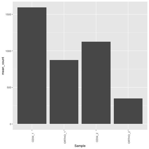
```

![](20191009_tidyr_files/figure-html/unnamed-chunk-93-1.png)

---
## forcats::fct_relevel - Reorder manually

```r
# fct_relevel - reorder manually
tidy_counts_expressed_norm %>% 
  ungroup() %>% 
  mutate_at(vars(Sample), as_factor) %>%
  mutate(Sample = fct_relevel(Sample, my_levels1)) %>% 
  pull(Sample) %>% head(n=10)
```

```
##  [1] CD34_1  ORTHO_1 CD34_2  ORTHO_2 CD34_1  ORTHO_1 CD34_2  ORTHO_2 CD34_1  ORTHO_1
## Levels: ORTHO_1 ORTHO_2 CD34_1 CD34_2
```

```
##  [1] CD34_1  ORTHO_1 CD34_2  ORTHO_2 CD34_1  ORTHO_1 CD34_2  ORTHO_2 CD34_1  ORTHO_1
## Levels: ORTHO_1 CD34_1 CD34_2 ORTHO_2
```
---
## forcats::fct_reorder - Reorder using data

```r
# fct_reorder - reorder based on the data. Here we are ordering based
# on mean counts for each sample.
tidy_counts_expressed_norm %>%
  ungroup() %>% 
  mutate_at(vars(Sample), as_factor) %>% 
  mutate(Sample = fct_reorder(Sample, counts, mean)) %>% 
  pull(Sample) %>% head(n=10)
```

```
##  [1] CD34_1  ORTHO_1 CD34_2  ORTHO_2 CD34_1  ORTHO_1 CD34_2  ORTHO_2 CD34_1  ORTHO_1
## Levels: ORTHO_2 ORTHO_1 CD34_2 CD34_1
```

---
## Now our ordering can be fixed

```r
p <- tidy_counts_expressed_norm %>% 
 ungroup() %>% 
 mutate_at(vars(Sample), as_factor) %>%
 mutate(Sample=fct_relevel(Sample, my_levels1)) %>% 
 group_by(Sample) %>% 
 summarize(mean_count=mean(counts)) %>% 
 ggplot(aes(x=Sample, y= mean_count)) + 
 geom_bar(stat = "identity") + 
 theme(axis.text.x = element_text(angle = 90))
```
---
## Now our ordering can be fixed

```r
p
```

![](20191009_tidyr_files/figure-html/unnamed-chunk-97-1.png)

---
## forcats::fct_recode - Change levels

```r
df1$age_classbylength
```

```
##  [1] "yearling"           "juvenile"           "juvenile"           "juvenile"          
##  [5] "juvenile"           "mixed age juvenile" "juvenile"           "juvenile"          
##  [9] "juvenile"           "juvenile"           "juvenile"           "juvenile"          
## [13] "juvenile"           "juvenile"           "juvenile"           "juvenile"          
## [17] "juvenile"           "juvenile"           "juvenile"           "juvenile"          
## [21] "juvenile"           "juvenile"           "juvenile"           "juvenile"          
## [25] "juvenile"           "juvenile"           "juvenile"           "juvenile"          
## [29] "juvenile"           "juvenile"           "yearling"           "yearling"          
## [33] "juvenile"           "yearling"           "mixed age juvenile" "juvenile"          
## [37] "juvenile"           "juvenile"           "juvenile"           "juvenile"          
## [41] "juvenile"           "juvenile"           "yearling"           "yearling"          
## [45] "yearling"           "yearling"           "yearling"           "yearling"          
## [49] "yearling"           "yearling"           "yearling"           "yearling"          
## [53] "yearling"           "yearling"           "yearling"           "yearling"          
## [57] "yearling"           "yearling"           "subyearling"        "juvenile"          
## [61] "juvenile"           "juvenile"           "juvenile"           "juvenile"          
## [65] "juvenile"           "yearling"           "juvenile"           "juvenile"          
## [69] "mixed age juvenile" "yearling"           "yearling"           "yearling"          
## [73] "yearling"           "yearling"           "yearling"           "yearling"          
## [77] "yearling"           "juvenile"           "juvenile"           "juvenile"          
## [81] "juvenile"           "juvenile"           "yearling"           "yearling"          
## [85] "yearling"           "yearling"           "yearling"           "yearling"          
## [89] "yearling"           "yearling"           "yearling"           "yearling"          
## [93] "yearling"           "yearling"           "yearling"           "yearling"          
## [97] "yearling"
```

```r
# Recoding levels to give them a new name
df1 %>% 
  mutate_at(vars(age_classbylength), as_factor) %>%
  mutate(age_classbylength=fct_recode(age_classbylength, "mixed juvenile" = "mixed age juvenile")) %>%
  pull(age_classbylength)
```

```
##  [1] yearling       juvenile       juvenile       juvenile       juvenile       mixed juvenile
##  [7] juvenile       juvenile       juvenile       juvenile       juvenile       juvenile      
## [13] juvenile       juvenile       juvenile       juvenile       juvenile       juvenile      
## [19] juvenile       juvenile       juvenile       juvenile       juvenile       juvenile      
## [25] juvenile       juvenile       juvenile       juvenile       juvenile       juvenile      
## [31] yearling       yearling       juvenile       yearling       mixed juvenile juvenile      
## [37] juvenile       juvenile       juvenile       juvenile       juvenile       juvenile      
## [43] yearling       yearling       yearling       yearling       yearling       yearling      
## [49] yearling       yearling       yearling       yearling       yearling       yearling      
## [55] yearling       yearling       yearling       yearling       subyearling    juvenile      
## [61] juvenile       juvenile       juvenile       juvenile       juvenile       yearling      
## [67] juvenile       juvenile       mixed juvenile yearling       yearling       yearling      
## [73] yearling       yearling       yearling       yearling       yearling       juvenile      
## [79] juvenile       juvenile       juvenile       juvenile       yearling       yearling      
## [85] yearling       yearling       yearling       yearling       yearling       yearling      
## [91] yearling       yearling       yearling       yearling       yearling       yearling      
## [97] yearling      
## Levels: yearling juvenile mixed juvenile subyearling
```

```r
# Recoding levels to change to add one factor to another factor
df1 %>% 
  mutate_at(vars(age_classbylength), as_factor) %>% 
  mutate(age_classbylength=fct_recode(age_classbylength, "juvenile" = "mixed age juvenile")) %>%
  pull(age_classbylength)
```

```
##  [1] yearling    juvenile    juvenile    juvenile    juvenile    juvenile    juvenile    juvenile   
##  [9] juvenile    juvenile    juvenile    juvenile    juvenile    juvenile    juvenile    juvenile   
## [17] juvenile    juvenile    juvenile    juvenile    juvenile    juvenile    juvenile    juvenile   
## [25] juvenile    juvenile    juvenile    juvenile    juvenile    juvenile    yearling    yearling   
## [33] juvenile    yearling    juvenile    juvenile    juvenile    juvenile    juvenile    juvenile   
## [41] juvenile    juvenile    yearling    yearling    yearling    yearling    yearling    yearling   
## [49] yearling    yearling    yearling    yearling    yearling    yearling    yearling    yearling   
## [57] yearling    yearling    subyearling juvenile    juvenile    juvenile    juvenile    juvenile   
## [65] juvenile    yearling    juvenile    juvenile    juvenile    yearling    yearling    yearling   
## [73] yearling    yearling    yearling    yearling    yearling    juvenile    juvenile    juvenile   
## [81] juvenile    juvenile    yearling    yearling    yearling    yearling    yearling    yearling   
## [89] yearling    yearling    yearling    yearling    yearling    yearling    yearling    yearling   
## [97] yearling   
## Levels: yearling juvenile subyearling
```
---
## forcats::fct_count() - Summarise by counting

```r
# fct_count - Count up the number of each
df1 %>% 
  mutate_at(vars(age_classbylength), as_factor) %>% 
  pull(age_classbylength) %>% 
  fct_count()
```

```
## # A tibble: 4 x 2
## f n
## <fct> <int>
## 1 yearling 44
## 2 juvenile 49
## 3 mixed age juvenile 3
## 4 subyearling 1
```
---
## forcats::fct_infreq() - Mask rare factors

```r
# fct_infreq - mask rare factors by giving them a general summary term i.e. Other
df1 %>% 
  mutate_at(vars(age_classbylength), as_factor) %>%
  mutate(age_classbylength=fct_lump(age_classbylength, n=2)) %>%
  pull(age_classbylength)
```

```
##  [1] yearling juvenile juvenile juvenile juvenile Other    juvenile juvenile juvenile juvenile
## [11] juvenile juvenile juvenile juvenile juvenile juvenile juvenile juvenile juvenile juvenile
## [21] juvenile juvenile juvenile juvenile juvenile juvenile juvenile juvenile juvenile juvenile
## [31] yearling yearling juvenile yearling Other    juvenile juvenile juvenile juvenile juvenile
## [41] juvenile juvenile yearling yearling yearling yearling yearling yearling yearling yearling
## [51] yearling yearling yearling yearling yearling yearling yearling yearling Other    juvenile
## [61] juvenile juvenile juvenile juvenile juvenile yearling juvenile juvenile Other    yearling
## [71] yearling yearling yearling yearling yearling yearling yearling juvenile juvenile juvenile
## [81] juvenile juvenile yearling yearling yearling yearling yearling yearling yearling yearling
## [91] yearling yearling yearling yearling yearling yearling yearling
## Levels: yearling juvenile Other
```

```r
df1 %>% 
  mutate_at(vars(age_classbylength), as_factor) %>%
  mutate(age_classbylength=fct_lump(age_classbylength, n=2)) %>%
  pull(age_classbylength) %>% 
  fct_count()
```

```
## # A tibble: 3 x 2
## f n
## <fct> <int>
## 1 yearling 44
## 2 juvenile 49
## 3 Other 4
```
---
## forcats::fct_c - Combining factors

```r
# Normally facotrs do not like to be combined as levels in one may not exist in the other.
# Factor concatenation with fct_c help get around this. 
A <- factor(c('Tom','Ji-Dung'))
B <- factor('Matt')
fct_c(A, B)
```

```
## [1] Tom     Ji-Dung Matt   
## Levels: Ji-Dung Tom Matt
```

---
## CHALLENGE: Time for an exercise!

Exercise reviewing purrr can be found [here](http://rockefelleruniversity.github.io/RU_tidyverse/tidyR/exercises/EX10_RU_tidyverse_forcats.html)

---
### Answers to exercise.

Answers can be found [here](http://rockefelleruniversity.github.io/RU_tidyverse/tidyR/answers/EX10_ANSWERS_RU_tidyverse_forcats.html)

R code for solutions can be found [here](http://rockefelleruniversity.github.io/RU_tidyverse/tidyR/answers/EX10_ANSWERS_RU_tidyverse_forcats.R)

---
# Summary 
We have covered the core packages in the tidyverse

* ~~ggplot2 – making pretty graphs~~ 
* ~~readr – reading data into R~~  
* ~~dplyr – manipulating data~~  
* ~~tibble - working with tibbles~~  
* ~~tidyr – miscellaneous tools for tidying data~~
* ~~purrr - iterating over data~~
* ~~stringr – working with strings~~  
* ~~forcats - working with factors~~

---
## Tidy beyond this workshop

Hadley Wickham (Chief Scientist at RStudio) is the driving force behind the tidyverse.

Hadley wrote a paper about why he thinks tidy data is best: www.jstatsoft.org/v59/i10/paper.

There is a lot of support for all things tidy at: https://www.tidyverse.org/  
(This includes really great cheat sheets for each tool)

---
## Tidy packages to check out:

plyranges: dplyr equivalent for working with ranges i.e. Granges

profileplyr: graphical and heatmap outputs for genomics

readxl: This package is very useful when you want to import Excel sheets in R

googledrive: Interact with your googledrive through R

lubridate and hms: Allow managin of calendar and time formats

magrittr: piping tools

broom: helps tidy up standard base function i.e. lm or t.test

tidymodels: A collection of tools for preparing for and validating model functions

---
## Other Good Resources

ggplot  
https://rockefelleruniversity.github.io/Plotting_In_R/

R for Data Science text book  
https://r4ds.had.co.nz/

Data Science with R text book   
http://garrettgman.github.io/

Biounformatics Shared Training - Intermediate R course   
https://bioinformatics-core-shared-training.github.io/r-intermediate/