Viz_part_2.utf8

class: center, middle, inverse, title-slide

# Visualizing Genomics Data (part 2)
<html>
<div style="float:left">

</div>
<hr color='#EB811B' size=1px width=796px>
</html>
### <a href="http://rockefelleruniversity.github.io/RU_VisualizingGenomicsData/" class="uri">http://rockefelleruniversity.github.io/RU_VisualizingGenomicsData/</a>

---

---
##Reminder of file types

In this session we will be dealing with a range of data types. For more information on file types you can revisit our material. 
 
* [File Formats](https://rockefelleruniversity.github.io/Genomic_Data/). 
 
For more information on visualizing genomics data in browsers you can visit our IGV course. 
 
* [IGV](https://rockefelleruniversity.github.io/IGV_course/). 
---
##Reminder of data types in Bioconductor

We will also encounter and make use of many data structures and data types which we have seen throughout our courses on HTS data. You can revisit this material to refresh on HTS data analysis in Bioconductor and R below. 
 
* [Bioconductor](https://rockefelleruniversity.github.io/Bioconductor_Introduction/)
* [Genomic Intervals](https://rockefelleruniversity.github.io/Bioconductor_Introduction/presentations/singlepage/GenomicIntervals_In_Bioconductor.html)
* [Genomic Scores](https://rockefelleruniversity.github.io/Bioconductor_Introduction/presentations/singlepage/GenomicScores_In_Bioconductor.html)
* [Sequences](https://rockefelleruniversity.github.io/Bioconductor_Introduction/presentations/singlepage/SequencesInBioconductor.html)
* [Gene Models](https://rockefelleruniversity.github.io/Bioconductor_Introduction/presentations/singlepage/GenomicFeatures_In_Bioconductor.html)
* [Alignments](https://rockefelleruniversity.github.io/Bioconductor_Introduction/presentations/singlepage/AlignedDataInBioconductor.html)
* [ChIP-seq](http://rockefelleruniversity.github.io/RU_ChIPseq/)
* [ATAC-seq](http://rockefelleruniversity.github.io/RU_ATACseq/)
* [RNA-seq](http://rockefelleruniversity.github.io/RU_RNAseq/)
 
---
##Materials

All material for this course can be found on github. 
* [Visualizing Genomics Data](https://github.com/RockefellerUniversity/RU_VisualizingGenomicsData) 
 
Or can be downloaded as a zip archive from here.  
* [Download zip](https://github.com/RockefellerUniversity/RU_VisualizingGenomicsData/archive/master.zip)

---
##Materials

Once the zip file in unarchived. All presentations as HTML slides and pages, their R code and HTML practical sheets will be available in the directories underneath. 
 
* **r_course/presentations/Slides/** 
Presentations as an HTML slide show. 
* **r_course/presentations/exercises/** 
Some tasks/examples to work through.

---
##Materials

All data to run code in the presentations and in the practicals is available in the zip archive. This includes coverage as bigWig files, aligned reads as BAM files and genomic intervals stored as BED files. 
 
We also include some RData files containing precompiled results from querying database (in case of external server downtime).

All data can be found under the **data** directory 
 
**data/** 
 
---
##Set the Working directory

Before running any of the code in the practicals or slides we need to set the working directory to the folder we unarchived.  
 
You may navigate to the unarchived visualizingGenomicsData folder in the Rstudio menu 
 
**Session -> Set Working Directory -> Choose Directory** 
 
or in the console.

```r
setwd("/PathToMyDownload/VisualizingGenomicsData/r_course/") 
# e.g. setwd("~/Downloads/VisualizingGenomicsData/r_course") 
```
 
 
---
## Recap

We saw previously how we can create **GenomeAxisTrack** objects to represents scales and plot these using the **plotTracks()** functions.

```r
library(Gviz) 
genomeAxis <- GenomeAxisTrack(name="MyAxis") 
plotTracks(genomeAxis,from=100,to=10100) 
```

---
## Recap

We can create **DataTrack** objects from GRanges objects and plot these alongside our **GenomeAxisTrack** object using the **plotTracks()** functions.

```r
library(rtracklayer) 
allChromosomeCoverage <- import.bw("data/activatedReads.bw",
                                   as="GRanges") 
accDT <- DataTrack(allChromosomeCoverage,chomosome="chr17") 
plotTracks(c(accDT,genomeAxis), 
           from=47504051,to=47600688, 
           chromosome="chr17",type="hist")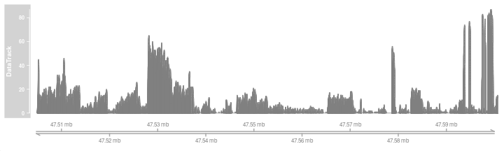 
```

![](Viz_part_2_files/figure-html/bbunny2-1.png)

---
## Recap

We created a **GeneRegionTrack** containing information on our gene models from our TxDb object and added this alongside data and axis to provide some context.

```r
library(TxDb.Mmusculus.UCSC.mm10.knownGene) 
customFromTxDb <- GeneRegionTrack(TxDb.Mmusculus.UCSC.mm10.knownGene,
                                  chromosome="chr17") 
plotTracks(c(accDT,customFromTxDb,genomeAxis), 
           from=47504051,to=47600688, 
           chromosome="chr17",type="hist")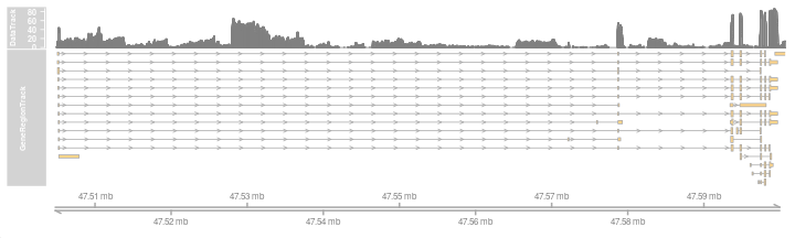 
```

![](Viz_part_2_files/figure-html/bbunny3-1.png)

---
##SequenceTracks 
 
When displaying genomics data it can be important to illustrate the underlying sequence for the genome being viewed. Gviz uses **SequenceTrack** objects to handle displaying sequencing information. 
 
First we need to get some sequence information for our genome of interest to display. Here we will use one of the **BSgenome** packages specific for hg19 - **BSgenome.Hsapiens.UCSC.hg19**. This contains the full sequence for hg19 as found in UCSC

```r
library(BSgenome.Hsapiens.UCSC.hg19) 
```

```
## Loading required package: BSgenome
```

```r
BSgenome.Hsapiens.UCSC.hg19[["chr7"]] 
```

```
## 159138663-letter DNAString object
## seq: NNNNNNNNNNNNNNNNNNNNNNNNNNNNNNNNNNNN...NNNNNNNNNNNNNNNNNNNNNNNNNNNNNNNNNNNN
```

---
##SequenceTracks

We can create a **SequenceTrack** object straight from this **BSgenome** object using the **SequenceTrack()** constructor. We can then plot this **SequenceTrack**, as with all tracks, using the **plotTracks()** functions. Here we specify the *from*, *to* and *chromosome* parameters to select a region to display.

```r
sTrack <- SequenceTrack(Hsapiens) 
```

```
## Warning:   Using providerVersion() on a BSgenome object is deprecated. Please use
##   'metadata(x)$genome' instead.
```

```r
plotTracks(sTrack,from=134887024,to=134887074, 
           chromosome = "chr7",cex=2.5) 
```

![](Viz_part_2_files/figure-html/unnamed-chunk-3-1.png)

---
##SequenceTracks from DNAstringset

We can also specify a DNAstringset object which we have encountered in the [Bioconductor](https://rockefelleruniversity.github.io/Bioconductor_Introduction/presentations/singlepage/SequencesInBioconductor.html) courses.

```r
dsSet <- DNAStringSet(Hsapiens[["chr7"]]) 
names(dsSet) <- "chr7" 
sTrack <- SequenceTrack(dsSet) 
plotTracks(sTrack,from=134887024,to=134887074, 
           chromosome = "chr7",cex=2.5) 
```

![](Viz_part_2_files/figure-html/unnamed-chunk-4-1.png)
 
---
##SequenceTracks from Fasta

We can also create our custom SequenceTrack from a [Fasta](https://rockefelleruniversity.github.io/Genomic_Data/genomicFileFormats.html#/) file. 
 
This fasta file just contains the same region we have used prior (chr7:134887024-134887074).

```r
sTrack <- SequenceTrack("data/chr7Short.fa") 
plotTracks(sTrack,from=1,to=50, 
           chromosome = "chr7",cex=2.5) 
```

![](Viz_part_2_files/figure-html/unnamed-chunk-6-1.png)

---
## Displaying complement sequence 
 
As with IGV, the sequence can be displayed as its complement. This is performed here by setting the **complement** argument to the **plotTracks()** function to TRUE/T.

```r
sTrack <- SequenceTrack("data/chr7Short.fa") 
plotTracks(sTrack,from=1,to=50, 
           chromosome = "chr7",complement=T,cex=2.5) 
```

![](Viz_part_2_files/figure-html/unnamed-chunk-7-1.png)

---
## Displaying strand information

We can also add 5' to 3' direction as we have for plotting **GenomeAxisTrack**  objects using the **add53** parameter. This allows for a method to illustrate the strand of the sequence being diplayed.

```r
sTrack <- SequenceTrack("data/chr7Short.fa") 
plotTracks(sTrack,from=1,to=50, 
           chromosome = "chr7",complement=F, 
           add53=T,cex=2.5) 
```

![](Viz_part_2_files/figure-html/unnamed-chunk-8-1.png)
---
## Displaying strand information 
 
Notice the 5' and 3' labels have swapped automatically when we have specified the complement sequence.

```r
sTrack <- SequenceTrack("data/chr7Short.fa") 
plotTracks(sTrack,from=1,to=50, 
           chromosome = "chr7",complement=T, 
           add53=T,cex=2.5) 
```

![](Viz_part_2_files/figure-html/unnamed-chunk-9-1.png)
---
## Controlling base display size

We can control the size of bases with the **cex** parameter, as with the standard R plotting.  
 
An interesting feature of this is that when plotted bases overlap, Gviz will provide a colour representation of bases instead of the bases' characters.

```r
plotTracks(sTrack,from=1,to=50, 
           chromosome = "chr7",cex=2.5) 
```

![](Viz_part_2_files/figure-html/unnamed-chunk-10-1.png)

```r
plotTracks(sTrack,from=1,to=50, 
           chromosome = "chr7", 
           cex=5) 
```

![](Viz_part_2_files/figure-html/unnamed-chunk-10-2.png)

---
## Controlling base display size

We can force the bases to be always a color representation instead of letter irrespective of **cex** by setting the **noLetters** parameter to **TRUE**.

```r
plotTracks(sTrack,from=1,to=50, 
           chromosome = "chr7",cex=1.1,noLetters=TRUE) 
```

![](Viz_part_2_files/figure-html/unnamed-chunk-11-1.png)
---
## Controlling base display size

If we want to color bases by own color scheme, we can provide a named vector of our desired colors to the *fontcolor* parameter.

```r
colForLetters <- c(A = "darkgrey", C = "red",
                    T = "darkgrey",G = "darkgrey")
plotTracks(sTrack,from=1,to=50, 
           chromosome = "chr7",cex=3,
           fontcolor=colForLetters) 
```

![](Viz_part_2_files/figure-html/unnamed-chunk-12-1.png)

---
## AlignmentsTrack

So far we have displayed summarized genomics data using GRange objects or GRanges with associated metadata. A prominent feature of Gviz is that it can work with genomic alignments, providing methods to generate graphical summaries on the fly. 
 
Genomic alignments are stored in Gviz within the AlignmentsTrack object. Here we can read genomic alignments in from a BAM file, see our file formats course material, by specifying its location.

```r
   peakReads <- AlignmentsTrack("data/small_Sorted_SRR568129.bam") 
   peakReads 
```

```
## ReferenceAlignmentsTrack 'AlignmentsTrack'
## | genome: NA
## | active chromosome: chrNA
## | referenced file: data/small_Sorted_SRR568129.bam
## | mapping: id=id, cigar=cigar, mapq=mapq, flag=flag, isize=isize, groupid=groupid, status=status, md=md, seq=seq
```

---
##AlignmentsTrack

The **AlignmentsTrack** object can be plotted in the same manner as tracks using **plotTracks()** function. 
 
Since the BAM file may contain information from all chromosomes we need to specify a chromsome to plot in the **chromosome** parameter and here we specify the **from** and **to** parameters too.

```r
   plotTracks(peakReads, 
              chromosome="chr5", 
              from=135312577, 
              to=135314146) 
```

![](Viz_part_2_files/figure-html/unnamed-chunk-14-1.png)

---
##AlignmentsTrack

```r
   plotTracks(peakReads, 
              chromosome="chr5", 
              from=135312577, 
              to=135314146) 
```

![](Viz_part_2_files/figure-html/unnamed-chunk-15-1.png)
 
 
By default **AlignmentTrack**s are rendered as both the reads themselves and the calculated coverage/signal depth from these reads. 
 
Reads, as with AnnotationTrack objects, show the strand of the aligned read by the direction of the arrow.

---
##AlignmentsTrack Plot Types
 
The type of plot/plots produced can be controlled by the **type** argument as we have done for **DataTrack** objects. 
 
The valid types of plots for AlignmentsTrack objects are "pileup", "coverage" and "sashimi" *(We've come across sashimi plots before)*.  
 
The type "pileup" displays just the reads.

```r
   plotTracks(peakReads, 
              chromosome="chr5", 
              from=135312577, 
              to=135314146, 
              type="pileup") 
```

![](Viz_part_2_files/figure-html/unnamed-chunk-16-1.png)
---
##AlignmentsTrack Plot Types

The type "coverage" displays just the coverage (depth of signal over genomic positions) calculated from the genomic alignments.

```r
   plotTracks(peakReads, 
              chromosome="chr5", 
              from=135312577, 
              to=135314146, 
              type="coverage") 
```

![](Viz_part_2_files/figure-html/unnamed-chunk-17-1.png)
---
##AlignmentsTrack Plot Types

As we have seen the default display is a combination of "pileup" and "coverage". 
 
We can provide multiple *type* arguments to the **plotTracks()** function as a vector of valid types. The order in vector *here* does not affect the display order in panels.

```r
   plotTracks(peakReads, 
              chromosome="chr5", 
              from=135312577, 
              to=135314146, 
              type=c("pileup","coverage")) 
```

![](Viz_part_2_files/figure-html/unnamed-chunk-18-1.png)
 
 
---
##AlignmentsTrack Plot Types

We have seen [sashimi plots in IGV](https://rockefelleruniversity.github.io/IGV_course/) when reviewing RNAseq data. 
 
Sashimi plots display the strength of signal coming from reads spanning splice junctions and so can act to illustrate changes in exon usage between samples. 
 
In IGV, we previous made use of the **BodyMap** data to show alternative splicing of an exon between heart and liver. 
 
<div align="center"> 
<img src="imgs/IGV_SplicingExample.png" alt="offset" height="400" width="800"> 
</div>

---
##AlignmentsTrack Plot Types

To recapitulate this plot, we have retrieved the subsection of **BodyMap** data as BAM files. 
 
First we must create two **AlignmentsTrack** objects, one for each tissue's BAM file of aligned reads.  
 
In this case since we are working with paired-end reads we must specify this by setting the **isPaired** parameter to TRUE

```r
heartReads <- AlignmentsTrack("data/heart.bodyMap.bam", 
                           isPaired = TRUE) 
liverReads <- AlignmentsTrack("data/liver.bodyMap.bam",  
                           isPaired = TRUE) 
 
liverReads 
```

```
## ReferenceAlignmentsTrack 'AlignmentsTrack'
## | genome: NA
## | active chromosome: chrNA
## | referenced file: data/liver.bodyMap.bam
## | mapping: id=id, cigar=cigar, mapq=mapq, flag=flag, isize=isize, groupid=groupid, status=status, md=md, seq=seq
```
---
##AlignmentsTrack Plot Types

As with **DataTrack** objects we can combine the **AlignmentTrack**s as a vector for plotting with the **plotTracks()** function. 
 
By default we will display the reads and calculated coverage. Here the paired reads and split reads are illustrated by thick and thin lines respectively.

```r
plotTracks(c(heartReads,liverReads), 
           chromosome="chr12", 
           from=98986825,to=98997877)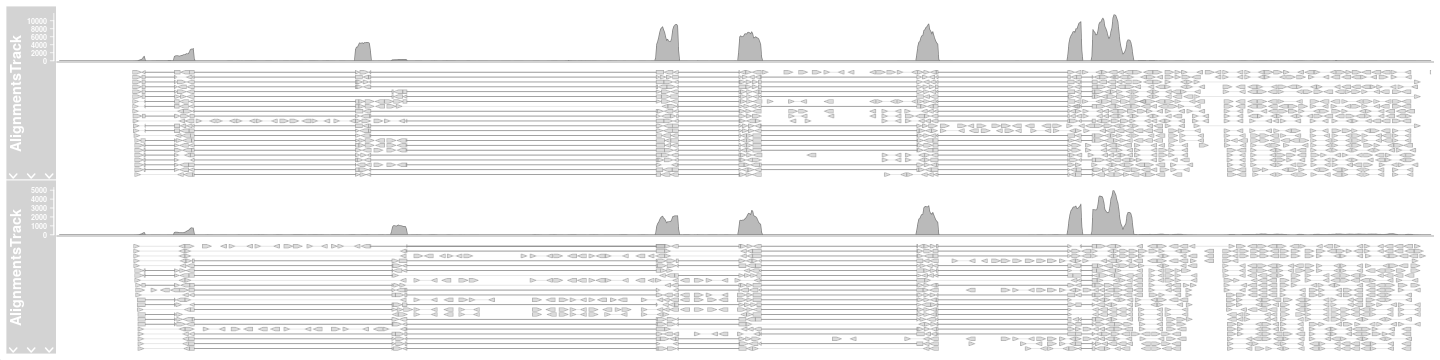 
```

![](Viz_part_2_files/figure-html/bb-1.png)
---
##AlignmentsTrack Plot Types

To reproduce a plot similar to that in IGV we can simply include the "sashimi" type in the **type** parameter vector, here alongside "coverage"

```r
plotTracks(c(heartReads,liverReads), 
           chromosome="chr12", 
           from=98986825, 
           to=98997877, 
           type=c("coverage","sashimi"))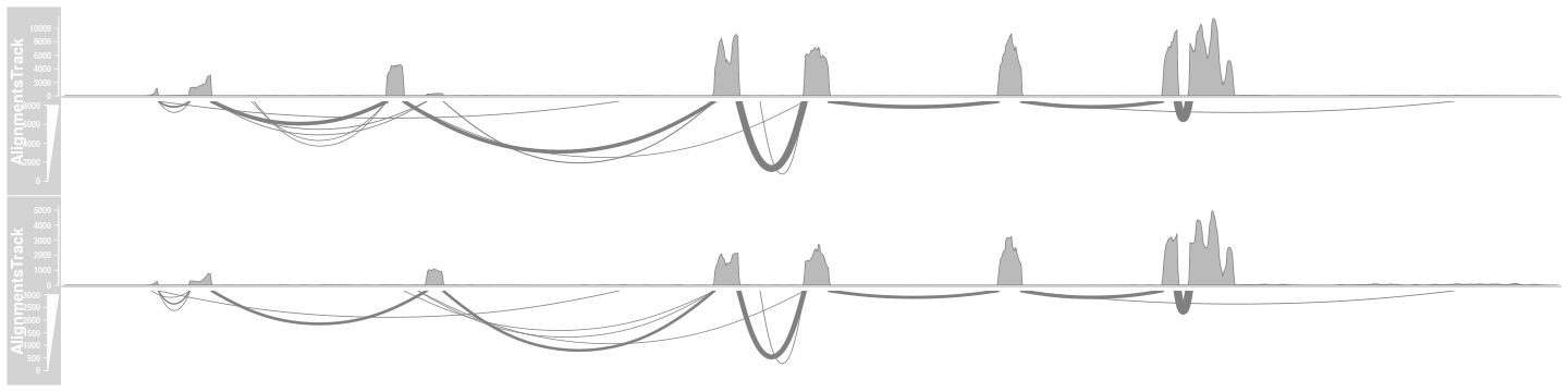 
```

![](Viz_part_2_files/figure-html/cc-1.png)

---
##AlignmentsTrack parameters

The **AlignmentTrack** object allows for specific parameters controlling how reads are displayed to be passed to the **plotTracks()** function. 
 
A few useful parameters are **col.gaps** and **col.mates** or **lty.gap** and **lty.mates** which will allow us to better distinguish between gapped alignments (split reads) and gaps between read pairs respectively.

```r
plotTracks(c(liverReads), 
           chromosome="chr12", 
           from=98986825,to=98997877, 
           col.gap="Red",col.mate="Blue")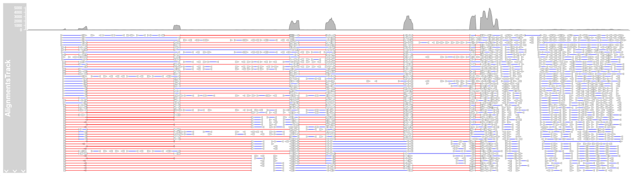 
```

![](Viz_part_2_files/figure-html/dd-1.png)
---
##AlignmentsTrack parameters 
 
Similarly using lty.gap and lty.mate parameters.

```r
plotTracks(c(liverReads), 
           chromosome="chr12", 
           from=98986825,to=98997877, 
           lty.gap=2,lty.mate=1)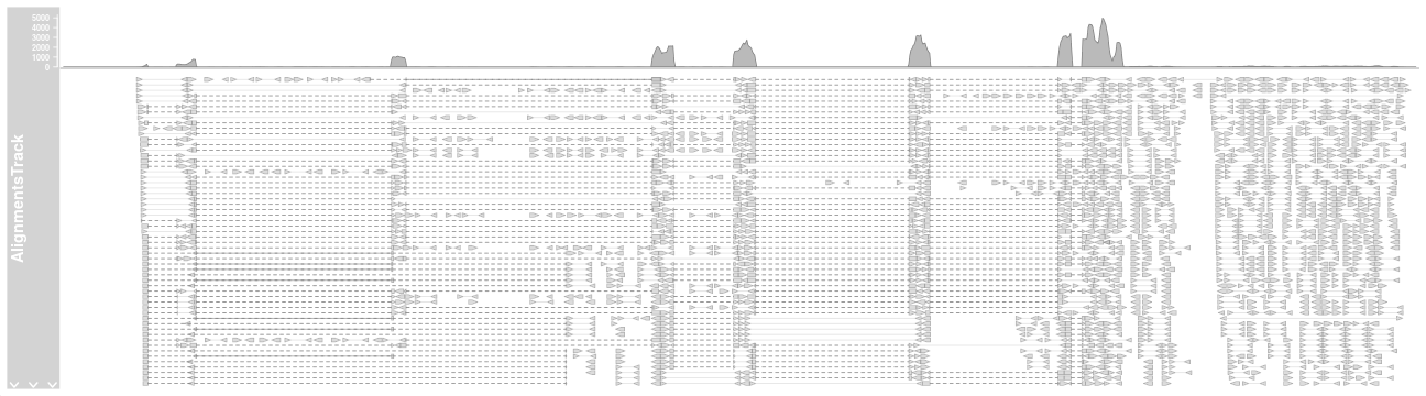 
```

![](Viz_part_2_files/figure-html/ee-1.png)
 
Line width may also be controlled with lwd.gap and lwd.mate parameters continuing the similarities to Base R plotting.

---
##AlignmentsTrack parameters

A common purpose in visualizing alignment data in browsers is review information relating to mismatches to the genome which may be related to SNPs. 
 
In order to highlight mismatches to the genome reference sequence we must first provide some information on the reference sequence. 
 
One method for this is to attach sequence information to the **AlignmentsTrack** itself by providing a **SequenceTrack** object to **referenceSequence** parameter in the **AlignmentsTrack()** constructor. Here we can create the **SequenceTrack** object ffor mouse.

```r
library(BSgenome.Mmusculus.UCSC.mm10)
sTrack <- SequenceTrack(BSgenome.Mmusculus.UCSC.mm10) 
```

```
## Warning:   Using providerVersion() on a BSgenome object is deprecated. Please use
##   'metadata(x)$genome' instead.
```

```r
activatedReads <- AlignmentsTrack("data/activatedSNPread.bam", 
                           isPaired = TRUE, 
                           referenceSequence=sTrack) 
```

---
##AlignmentsTrack parameters

Now when we can replot the pileup of reads where mismatches in the reads are highlighted.

```r
plotTracks(c(activatedReads,customFromTxDb), 
           chromosome="chr6", 
           from=124815373,to=124815412)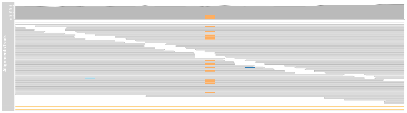 
```

![](Viz_part_2_files/figure-html/gg-1.png)

---
##AlignmentsTrack parameters
 
We could also specify the SequenceTrack in the **plotTracks()** function as shown for the liver reads example here. Here we simply include the relevant **SequenceTrack** object as a track to be plotted  alongside the BAM.

```r
plotTracks(c(activatedReads,sTrack), 
           chromosome="chr6", 
           from=124815373,to=124815412,cex=2)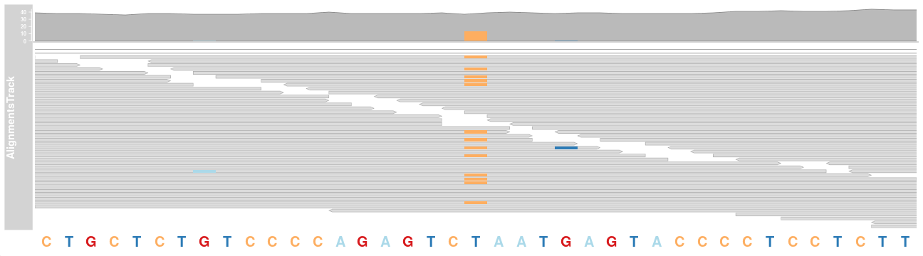 
```

![](Viz_part_2_files/figure-html/hh-1.png)

---
##Bringing in External data

**Gviz** has functions to allow us to import data from external repositories and databases. 
 
As in the IGV course, visualising genomics data in the context of additional genome information and external data held at these repositories provides a deeper insight into our own data. 
 
In this course we will look at two main methods of querying external databases- 
 
* The **BiomartGeneRegionTrack** object and constructor. 
* The **UcscTrack** object and constructor 
 
---
## Gene models through Biomart

The **biomaRt** Bioconductor package to programatically query various [Biomarts](http://useast.ensembl.org/biomart/martview/07c68e326d8ee955472140d9da19b959). 
 
**Gviz** allows us to both query Biomarts and automatically create a GeneRegionTrack using the **BiomartGeneRegionTrack** objects and **BiomartGeneRegionTrack()** constructor. 
---
##Gene models through Biomart

Here we construct a simple **BiomartGeneRegionTrack** object using the parameters to define locations of interest - "chromsome", "start", "end", "genome" as well as the Biomart to use, in this case Ensembl by setting the **name** parameter.

```r
bgrTrack <- BiomartGeneRegionTrack(genome="hg19", 
                                   start=26591341, 
                                   end=27034958, 
                                   chromosome = "7", 
                                   name="ENSEMBL") 
```
---
## Gene models through Biomart

We can then plot the BiomartGeneRegionTrack as we have previous GeneRegionTracks.

```r
plotTracks(bgrTrack)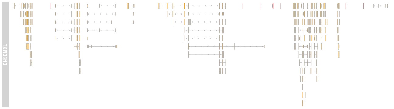 
```

![](Viz_part_2_files/figure-html/b-1.png)

---
## Gene models through Biomart

We can also specify filters in the **BiomartGeneRegionTrack()** constructor using the **filter** parameter. 
 
**Gviz** uses the **BiomaRt** Bioconductor package to query the Biomarts so we can review availble options using **BiomaRt's**  **useMart()** function to list available data collections and **listDatasets()** function to review all available datasets within the *ENSEMBL_MART_ENSEMBL* mart.

```r
library(biomaRt)
martList <- listMarts()
mart = useMart("ENSEMBL_MART_ENSEMBL")
dataList <- listDatasets(mart)
mart = useMart("ENSEMBL_MART_ENSEMBL", dataset="hsapiens_gene_ensembl") 
filterList <- listFilters(mart)
```

---
## Gene models through Biomart

Here we select only genes which have been annotated by both havana and ensembl (so called *Golden Transcripts*)

```r
bgrTrack_hav <- BiomartGeneRegionTrack(genome="hg19", 
                                   start=26591341, 
                                   end=27034958, 
                                   chromosome = "7", 
                                   name="ENSEMBL",               
                                  filter=list(source="ensembl_havana")) 
```

---
## Gene models through Biomart
 
Once we have retrieved our filtered gene models we can plot them as before.

```r
plotTracks(bgrTrack_hav) 
```

---
##Tracks from UCSC

A well known browser and source of genomic data and annotation is the [UCSC genome browser](https://genome.ucsc.edu/). **Gviz** can create track directly from UCSC tables using the functionality from **rtracklayer** Bioconductor package. 
 
The **Ucsctrack()** constructor and object allow for the query and track construction of a variety of data types. The **Ucsctrack()** function therefore requires us to specify the track type we expect using the **trackType** parameter as well as the required UCSC table using the **track** parameter.  
 
---
##Tracks from UCSC

To understand which tables are available we can query the **rtracklayer** package to identify track and table names.

We can use the **broswerSession()** function to connect to UCSC and the **genome()** function to establish the genome of interest. We can then review available tracks using the **trackNames()** function.

```r
library(rtracklayer) 
session <- browserSession() 
genome(session) <- "hg19" 
# trackNames(session) 
```

---
##Tracks from UCSC

We can identify available tables by using the **ucscTableQuery()** function and the **tableNames()** function.

```r
query <- ucscTableQuery(session, "Ensembl Genes", 
                        GRangesForUCSCGenome("hg19", "chr7", 
                                             IRanges(26591341,27034958))) 
tableNames(query) 
```

```
## [1] "ensGene"           "ccdsInfo"          "ensGtp"           
## [4] "ensPep"            "ensemblSource"     "ensemblToGeneName"
## [7] "knownToEnsembl"
```

---
##Tracks from UCSC

```r
ucscTrack <- UcscTrack(genome = "hg19", 
                       chromosome = "chr7", 
                       track = "ensGene", 
                       from = 26591341, 
                       to = 27034958, 
                       trackType = "GeneRegionTrack", 
                       rstarts = "exonStarts", 
                       rends = "exonEnds", 
                       gene ="name", 
                       symbol = "name2", 
                       transcript = "name", 
                       strand = "strand" 
) 
```

To build the UCSC annotation as a **GeneRegionTrack** we must specify some information specific to **GeneRegionTrack** objects. This includes the "rstarts" and "rends". You can consult the help for **GeneRegionTrack()** (*?GeneRegionTrack to see from in R*) to see full parameters required for **UcscTrack** objects.

---
##Tracks from UCSC

Now we can compare the Ensembl gene builds from the two different sources.  
 
Notable differences in the annotation include the absence of some transcripts due to the additional filter applied in our **BiomartGeneRegionTrack** object creation.

```r
plotTracks(c(bgrTrack,ucscTrack), 
           from = 26591341,to = 27034958) 
```

```
## Warning in plotTracks(c(bgrTrack, ucscTrack), from = 26591341, to = 27034958):
## The track chromosomes in 'trackList' differ. Setting all tracks to chromosome
## '7'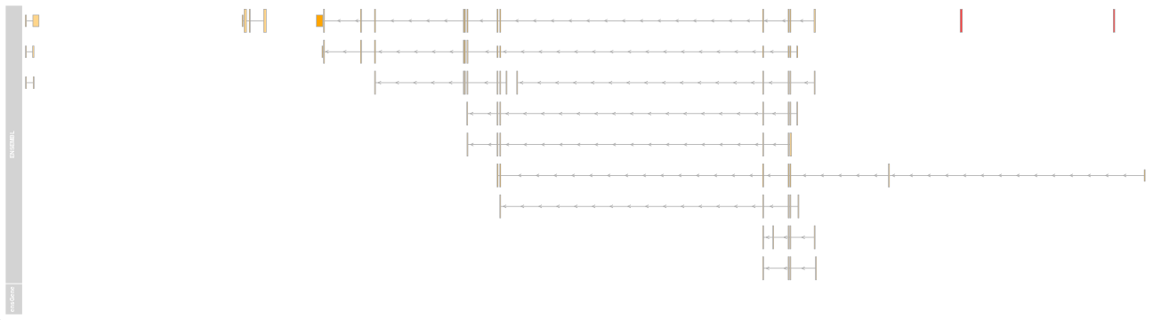
```

![](Viz_part_2_files/figure-html/e1-1.png)
 
---
##From UCSC to DataTracks

By the same method we can take advantage of other types of UCSC data. In this example we capture the Conservation in the phyloP100wayAll table over and around our previously investigated ChIPseq reads peak. 
 
Here we specify the data to be returned as a **DataTrack** object and the display type to be "hist". Here we are creating a **DataTrack** so would consult **DataTrack()** help *(?DataTrack)* to get full parameter list.

```r
conservationTrack <- UcscTrack(genome = "hg19",
                               chromosome = "chr5",
                               track = "Conservation",
                               table = "phyloP100wayAll",
                               from = 135313003,to = 135313570,
                               trackType = "DataTrack",
                               start = "start", end = "end", 
                               data = "score",type = "hist", window = "auto",
                               col.histogram = "darkblue",fill.histogram = "darkblue",
                               ylim = c(-3.7, 4),name = "Conservation") 
```
 
 
---
##From UCSC to DataTracks
 
With the inclusion of conservation alongside the coverage from CTCF peaks we can see a spike in conservation around the CTCF peak summit. We include a relative scale and increase the size of text for completeness.

```r
plotTracks(c(conservationTrack,peakReads,genomeAxis), 
           from=135313003, 
           to=135313570, 
           chromosome = "chr5", 
           type = c("hist","coverage"), 
           sizes = c(1,1,0.2), 
           cex=2)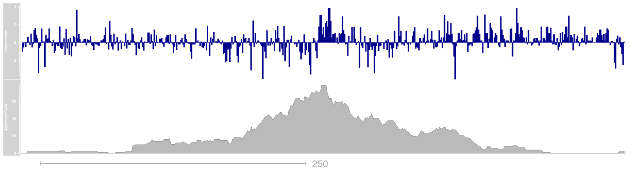 
```

![](Viz_part_2_files/figure-html/i1-1.png)
 
---
##Exercises

Time for exercises! [Link here](../../exercises/exercises/Viz_part2_exercise.html) 
 
---
##Solutions

Time for exercises! [Link here](../../exercises/answers/Viz_part2_answers.html)