ChIPseq_In_Bioconductor2.knit

class: center, middle, inverse, title-slide

# ChIPseq In Bioconductor (part2)
<html>
<div style="float:left">

</div>
<hr color='#EB811B' size=1px width=796px>
</html>
### Rockefeller University, Bioinformatics Resource Center
### <a href="http://rockefelleruniversity.github.io/RU_ChIPseq/" class="uri">http://rockefelleruniversity.github.io/RU_ChIPseq/</a>

---

## Data

In todays session we will continue to review the Myc ChIPseq we were working on in our last session.

This include Myc ChIPseq for MEL and Ch12 celllines as well as their input controls.

Information and files for the [Myc ChIPseq in MEL cell line can be found here](https://www.encodeproject.org/experiments/ENCSR000EUA/)

Information and files for the [Myc ChIPseq in Ch12 cell line can be found here](https://www.encodeproject.org/experiments/ENCSR000ERN/)

Input control can be found for [MEL cell line can be found here](https://www.encodeproject.org/experiments/ENCSR000ADN/)

Input control can be found for [Ch12 cell line can be found here.](https://www.encodeproject.org/experiments/ENCSR000ERS/)

---
class: inverse, center, middle

# Quality Control

---

## Quality Control

ChIPseq has many sources of potential noise including 
* Varying efficiency of antibodies
* Non-specific binding
* Library complexity
* ChIP artifacts and background

Many of these sources of noise can be assessed using some well established methodology.

---

# Quality Control References

For some discussions:

* Encode quality metrics.

[Large-scale quality analysis of published ChIPseq data. Marinov GK, Kundaje A, Park PJ, Wold BJ. G3 (Bethesda). 2014 Feb 19;4(2)](http://www.ncbi.nlm.nih.gov/pmc/articles/PMC3931556/)

* Overestimation of artefact duplicates in ChIPseq.

[Systematic evaluation of factors influencing ChIPseq fidelity.Nat Methods. Chen Y, Negre N, Li Q, Mieczkowska JO, Slattery M, Liu T, Zhang Y, Kim TK, He HH, Zieba J, Ruan Y, Bickel PJ, Myers RM, Wold BJ, White KP, Lieb JD, Liu XS. 2012 Jun;9(6)](http://www.ncbi.nlm.nih.gov/pmc/articles/PMC3477507/)

* When and what QC is useful.

[Impact of artifact removal on ChIP quality metrics in ChIPseq and ChIP-exo data.Front Genet. 2014 Apr 10;5:75.Carroll TS, Liang Z, Salama R, Stark R, de Santiago I](http://www.ncbi.nlm.nih.gov/pmc/articles/PMC3989762/)

---
## Always have an appropriate input

* Input samples are typically made from fragmented DNA prior to IP enrichment.

* Allows for control of artefact regions which occur across samples.

* NEVER run ChIPseq without considering which input to use.

For example: When using tumour samples for ChIPseq, it is important to have matched input samples. 
Differing conditions of same tissue may share common input.

---
## Quality metrics for ChIPseq

The [**ChIPQC package**](https://bioconductor.org/packages/release/bioc/html/ChIPQC.html) wraps some of the metrics into a Bioconductor package and takes care to measure these metrics under the appropriate condition.

To run a single sample we can use the **ChIPQCsample()** function, the relevant **unfiltered** BAM file and we are recommended to supply a **blacklist** as a BED file or GRanges and Genome name.

You can find a Blacklist for most genomes at [Anshul Kundaje's site](https://sites.google.com/site/anshulkundaje/projects/blacklists) or directly from the [Encode websites](https://www.encodeproject.org/annotations/ENCSR636HFF/)

```r
QCresult <- ChIPQCsample(reads = "/pathTo/myChIPreads.bam", genome = "mm10", blacklist = "/pathTo/mm10_Blacklist.bed")
```

---
## Quality control with ChIPQC

We download the blacklist for mm10 from [Encode ](https://www.encodeproject.org/files/ENCFF547MET/@@download/ENCFF547MET.bed.gz)

We can then provide an initial analysis of our ChIPseq samples quality using the **ChIPQCsample()** function from the [**ChIPQC** package.](http://bioconductor.org/packages/stats/bioc/ChIPQC/)

Here we evaluate the quality of samples we aligned in the prior session with Rsubread. The returned object is a **ChIPQCsample** object.

```r
library(ChIPQC)
toBlkList <- "~/Downloads/ENCFF547MET.bed.gz"
chipqc_MycMel_rep1 <- ChIPQCsample("SR_Myc_Mel_rep1.bam", annotation = "mm10", blacklist = toBlkList,
    chromosomes = paste0("chr", 1:10))
class(chipqc_MycMel_rep1)
```

```
## [1] "ChIPQCsample"
## attr(,"package")
## [1] "ChIPQC"
```

---
## Quality control with ChIPQC

We can display our **ChIPQCsample** object which will show a basic summary of our ChIPseq quality.

```r
chipqc_MycMel_rep1
```

```
## 					ChIPQCsample
```

```
## Number of Mapped reads: 10355431
```

```
## Number of Mapped reads passing MapQ filter: 8445736
```

```
## Percentage Of Reads as Non-Duplicates (NRF): 100(0)
```

```
## Percentage Of Reads in Blacklisted Regions: 8
```

```
## SSD: 4.15396194667776
```

```
## Fragment Length Cross-Coverage:
```

```
## Relative Cross-Coverage:
```

```
## Percentage Of Reads in GenomicFeature:
```

```
##                         ProportionOfCounts
## BlackList                       0.09376116
## LongPromoter20000to2000         0.39108812
## Promoters2000to500              0.06601580
## Promoters500                    0.05096595
## All5utrs                        0.02653351
## Alltranscripts                  0.73319436
## Allcds                          0.09148486
## Allintrons                      0.61883381
## All3utrs                        0.02559232
```

```
## Percentage Of Reads in Peaks: NA
```

```
## Number of Peaks: 0
```

```
## GRanges object with 0 ranges and 0 metadata columns:
##    seqnames    ranges strand
##       <Rle> <IRanges>  <Rle>
##   -------
##   seqinfo: no sequences
```

---
## QC of multiple samples

It is best to review ChIPseq quality versus your input controls and other Myc samples which we are using (or even external data if you do not have your own).

This will allow us to identify expected patterns of ChIPseq enrichment in our samples versus controls as well as spot any outlier samples by these metrics.

We can run **ChIPQCsample()** on all our samples of interest using an **lapply**.

```r
bamsToQC <- c("Sorted_Myc_Ch12_1.bam", "Sorted_Myc_Ch12_2.bam", "Sorted_Myc_MEL_1.bam",
    "Sorted_Myc_MEL_2.bam", "Sorted_Input_MEL.bam", "Sorted_Input_Ch12.bam")
myQC <- bplapply(bamsToQC, ChIPQCsample, annotation = "mm10", blacklist = toBlkList,
    chromosomes = paste0("chr", 1:10))
names(myQC) <- bamsToQC
```

---
## QC of multiple samples

All ChIPQC functions can work with a named list of **ChIPQCsample** objects to aggregate scores into table as well as plots.

Here we use the **QCmetrics()** function to give an overview of quality metrics.

```r
QCmetrics(myQC)
```

```
##                          Reads Map% Filt% Dup% ReadL FragL RelCC  SSD RiP%
## Sorted_Myc_Ch12_1.bam 10993821  100  21.9    0    35   186 1.070 3.82   NA
## Sorted_Myc_Ch12_2.bam 10060460  100  18.4    0    35   146 1.310 2.84   NA
## Sorted_Myc_MEL_1.bam  10111080  100  20.8    0    35   177 1.220 3.42   NA
## Sorted_Myc_MEL_2.bam  10686984  100  23.4    0    35   177 1.050 4.20   NA
## Sorted_Input_MEL.bam   8591703  100  23.6    0    36   184 0.620 4.51   NA
## Sorted_Input_Ch12.bam 10429244  100  23.7    0    35   182 0.275 4.26   NA
##                       RiBL%
## Sorted_Myc_Ch12_1.bam  12.8
## Sorted_Myc_Ch12_2.bam  10.1
## Sorted_Myc_MEL_1.bam   11.9
## Sorted_Myc_MEL_2.bam   14.0
## Sorted_Input_MEL.bam   15.9
## Sorted_Input_Ch12.bam  12.8
```

---
class: inverse, center, middle

# Assessing fragment length

---

## Assessing fragment length

The prediction of fragment length is an essential part of ChIPseq affecting peaks calling, summit identification and coverage profiles.

The use of cross-correlation or cross-coverage allows for an assessment of reads clustering by strand and so a measure of quality.

---
## Assessing fragment length

---

## Assessing fragment length

* In ChIPseq typically short single end reads of dsDNA.

* **dsDNA single end sequencing means**
+ 5' of fragment will be sequenced on "+" strand
+ 3' of fragment end will be on "-" strand.

* **Although we only have partial sequence of strand, with predicted fragment length we can predict the whole fragment**
+ "+" reads should extend only in positive direction 
+ "-" reads only in negative

---

## Assessing fragment length

---

## Assessing fragment length

---

## Assessing fragment length

---

## Cross-coverage plot

---

## Cross-coverage plot
The **plotCC** function can be used to plot our cross-coverage profiles

The **plotCC()** function accepts our list of ChIPQC sample objects and a **facetBy** argument to allow us to group our cross-coverage profiles.

```r
plotCC(myQC, facetBy = "Sample")
```

![](ChIPseq_In_Bioconductor2_files/figure-html/qcmetridedecs-1.png)

---

## Cross-coverage plot

We can include metadata as a data.frame where the first column is our sample names to allow us to group our plot in different ways.

```r
myMeta <- data.frame(Sample = names(myQC), Tissue = c("Ch12", "Ch12", "MEL", "MEL",
    "MEL", "Ch12"), Antibody = c(rep("Myc", 4), rep("Input", 2)))
myMeta
```

```
##                  Sample Tissue Antibody
## 1 Sorted_Myc_Ch12_1.bam   Ch12      Myc
## 2 Sorted_Myc_Ch12_2.bam   Ch12      Myc
## 3  Sorted_Myc_MEL_1.bam    MEL      Myc
## 4  Sorted_Myc_MEL_2.bam    MEL      Myc
## 5  Sorted_Input_MEL.bam    MEL    Input
## 6 Sorted_Input_Ch12.bam   Ch12    Input
```

---
## Cross-coverage plot

We can now include our metadata to the **addMetaData** argument which will allow us to **facetBy** the supplied metadata columns.

Additionally here we use the **colourBy** parameter to add colour to antibody groups.

```r
plotCC(myQC, facetBy = "Tissue", addMetaData = myMeta, colourBy = "Antibody")
```

![](ChIPseq_In_Bioconductor2_files/figure-html/qcmetricsede-1.png)

---
## Cross-coverage plot

All plots in ChIPQC are in fact built in ggplot2 so we can edit and update our plot like all ggplot objects.

```r
plotCC(myQC, facetBy = "Tissue", addMetaData = myMeta, colourBy = "Antibody") + theme_bw() +
    ggtitle("ChIPQC results")
```

![](ChIPseq_In_Bioconductor2_files/figure-html/qcmetricsrf-1.png)

---
class: inverse, center, middle

# Blacklists and SSD

---

## Blacklists

ChIPseq will often show the presence of common artifacts, such as ultra-high signal regions. Such regions can confound peak calling, fragment length estimation and QC metrics. Anshul Kundaje created the DAC blacklist as a reference to help deal with these regions.

---
## Blacklist affects many metrics

---
## Blacklists and SSD

SSD is one of these measures that is sensitive to blacklisted artifacts. SSD is a measure of standard deviation of signal across the genome with higher scores reflecting significant pile-up of reads. SSD can therefore be used to assess both the extent of ultra high signals and the signal. But first blacklisted regions must be removed.

---
## Standardized Standard Deviation

ChIPQC calculates SSD before and after removing signal coming from Blacklisted regions.

The **plotSSD()** function plots samples's pre-blacklisting score in **red** and post-blacklisting score in **blue**.

Higher scores for pre-blacklisted SSD can suggest a strong background signal in blacklisted regions for that sample.

```r
plotSSD(myQC) + xlim(0, 5)
```

![](ChIPseq_In_Bioconductor2_files/figure-html/unnamed-chunk-8-1.png)

---
## Standardized Standard Deviation

Since SSD score is strongly affected by blacklisting it may be necessary to change the axis to see any differences between samples for post-blacklisting scores.

Higher post-blacklisted SSD scores reflect samples with stronger peak signal.

```r
plotSSD(myQC) + xlim(0.2, 0.8)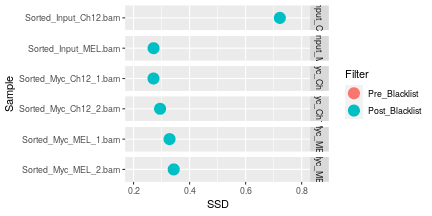
```

![](ChIPseq_In_Bioconductor2_files/figure-html/unnamed-chunk-9-1.png)

---
class: inverse, center, middle

# Library complexity and enrichment

---

## Library complexity

A potential source of noise in ChIPseq is overamplification of the ChIPseq library during a PCR step. This can lead to large number of duplicate reads which may confound peak calling.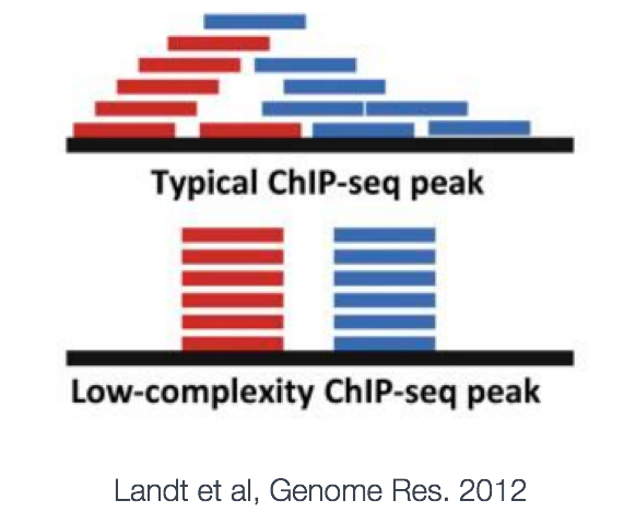

![](imgs/mappable.png)

---
## Duplication

We should compare our duplication rate across samples to identify any sample experiencing overamplification and so potential of a lower complexity.

The **flagtagcounts()** function reports can report the number of duplicates and total mapped reads and so from there we can calculate our duplication rate.

```r
myFlags <- flagtagcounts(myQC)
myFlags["DuplicateByChIPQC", ]/myFlags["Mapped", ]
```

```
## Sorted_Myc_Ch12_1.bam Sorted_Myc_Ch12_2.bam  Sorted_Myc_MEL_1.bam 
##            0.07203883            0.08633293            0.15987076 
##  Sorted_Myc_MEL_2.bam  Sorted_Input_MEL.bam Sorted_Input_Ch12.bam 
##            0.06253850            0.14269010            0.13873057
```

---
## Enrichment for reads across genes

We can also use ChIPQC to review where our distribution of reads across gene features using the **plotRegi()** function.

Here we expect ChIPseq signal to be stronger in 5'UTRs and promoters when compared to input samples.

```r
p <- plotRegi(myQC)
```

---
## Enrichment for reads across genes.

```r
p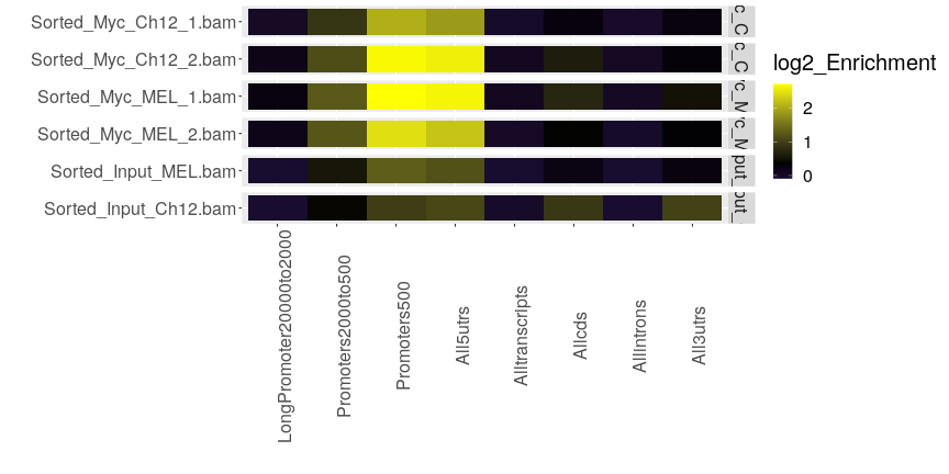
```

![](ChIPseq_In_Bioconductor2_files/figure-html/unnamed-chunk-13-1.png)

---
class: inverse, center, middle

# Peak Calling

---

## Peak calling

To identify regions of Myc transcription factor binding we can use a **peak caller**.

Although many peak callers are available in R and beyond, the most popular and widely used peak caller remains **MACS2**.

MACS2 calls peaks in a few simple steps.

* Predict fragment length.
* Shift reads to center of predicted fragment.
* Scan across genome and identify regions enriched compare to control samples using count based statistic.

---
## Installing programs that aren't in R

There is no R package for MACS2 (well it just got [released](https://github.com/macs3-project/MACS) but we haven't tested it yet). It is possible to install it on Mac and Linux using the [Anaconda](https://anaconda.org/bioconda/macs2) package repository (unfortunately there is not a Windows implementation). Anaconda is a huge collection of version controlled packages that can be installed through the conda package management system. With conda it is easy to create and manage environments that have a variety of different packages in them.

Though there is no MACS2 R package, we can interact with the anaconda package system using the R package [Herper](https://bioconductor.org/packages/release/bioc/html/Herper.html). This was created by us here at the BRC and is part of Bioconductor.

```r
BiocManager::install("Herper")
library(Herper)
```

---
## Install MACS2 with Herper

First, we will use Herper to install MACS2 with the *install_CondaTools* function. We just need to tell *install_CondaTools* what tool/s you want and the name of the environment you want to build.

```r
salmon_paths <- install_CondaTools(tools = "macs2", env = "ChIPseq_analysis")
salmon_paths
```

Behind the scenes, Herper will install the most minimal version of conda (called miniconda), and then will create a new environment into which MACS2 will be installed. When you run the function it prints out where MACS2 is installed. There are additional arguments to control where miniconda is installed using *pathToMiniConda* and also update an existing environment with *updateEnv*.

---
## Running MACS2

To run MACS2 to we simply need to supply.

* A BAM file to find enriched regions in. (specified after **-t**)
* A Name for peak calls (specified after **–name**).
* An output folder to write peaks into (specified after **–outdir**).
* Optionally, but highly recommended, we can identify a control to compare to (specified after **–c**).

```bash
macs2 callpeak -t Sorted_Myc_MEL_1.bam
               –name Mel_Rep1 
               –-outdir PeakDirectory
               -c Sorted_Input_MEL.bam

```

---
## Running MACS2 in R

Herper allows us to run conda packages from within R. MACS2 has been installed into *ChIPseq_analysis*. So we can use this environment from R using *with_CondaEnv()*.

```r
myChIP <- "Sorted_Myc_MEL_1.bam"
myControl <- "Sorted_Input_MEL.bam"

with_CondaEnv("ChIPseq_analysis",
                      system2(command="macs2",args =c("callpeak", 
                      "-t", myChIP,
                      "-n", "Mel_Rep1",
                      "–-outdir","PeakDirectory",
                      "-c", myControl)),
                        
                        stdout = TRUE))
```

---
## Working with Peaks

MACS peak calls can be found in our specied output directory with the suffix and extension "_peaks.xls".

MACS peaks come as a tab seperated file thinly disguised as a ".xls".

In addition to the genomic coordinates of peaks, these files contain useful information on the samples, parameters and version used for peak calling at the top.

```r
macsPeaks <- "data/Mel1_peaks.xls"

macsPeaks_DF <- read.delim(macsPeaks)
macsPeaks_DF[1:8, ]
## [1] "# Command line: callpeak -t Sorted_Myc_MEL_1.bam -n Mel1 -c Sorted_Input_MEL.bam"
## [2] "# ARGUMENTS LIST:"                                                               
## [3] "# name = Mel1"                                                                   
## [4] "# format = AUTO"                                                                 
## [5] "# ChIP-seq file = ['Sorted_Myc_MEL_1.bam']"                                      
## [6] "# control file = ['Sorted_Input_MEL.bam']"                                       
## [7] "# effective genome size = 2.70e+09"                                              
## [8] "# band width = 300"
```

---

## Importing MACS peaks

We can import peak files therefore using read.delim function. Note we have set comment.char argument to **#** to exclude additional information on peak calling parameters stored within the MACS peak file.

```r
macsPeaks <- "data/Mel1_peaks.xls"

macsPeaks_DF <- read.delim(macsPeaks, comment.char = "#")
macsPeaks_DF[1:2, ]
##    chr   start     end length abs_summit pileup X.log10.pvalue. fold_enrichment
## 1 chr1 4785371 4785642    272    4785563  20.89        10.66553         5.33590
## 2 chr1 5082993 5083247    255    5083123  33.42        12.68072         4.30257
##   X.log10.qvalue.        name
## 1         7.37727 Mel1_peak_1
## 2         9.27344 Mel1_peak_2
```

---

## Converting MACS peaks

Now we have the information in a table we can create a GRanges object.

GRanges objects are made of chromosome names and intervals stored as IRanges.

```r
library(GenomicRanges)
macsPeaks_GR <- GRanges(seqnames = macsPeaks_DF[, "chr"], IRanges(macsPeaks_DF[,
    "start"], macsPeaks_DF[, "end"]))
macsPeaks_GR
## GRanges object with 16757 ranges and 0 metadata columns:
##           seqnames            ranges strand
##              <Rle>         <IRanges>  <Rle>
##       [1]     chr1   4785371-4785642      *
##       [2]     chr1   5082993-5083247      *
##       [3]     chr1   7397544-7398115      *
##       [4]     chr1   7616290-7616433      *
##       [5]     chr1   8134747-8134893      *
##       ...      ...               ...    ...
##   [16753]     chrY   2657144-2657294      *
##   [16754]     chrY 90784142-90784289      *
##   [16755]     chrY 90818471-90818771      *
##   [16756]     chrY 90824549-90824905      *
##   [16757]     chrY 90825407-90825575      *
##   -------
##   seqinfo: 21 sequences from an unspecified genome; no seqlengths
```

---
## Peaks as GRanges

As we have seen before elements in GRanges can accessed and set using various GRanges functions.
Here we can deconstruct our object back to contig names and interval ranges.

```r
seqnames(macsPeaks_GR)
```

```
## factor-Rle of length 16757 with 21 runs
##   Lengths:   916   822  1795   582   596 ...  1089   836   954   395     7
##   Values : chr1  chr10 chr11 chr12 chr13 ... chr7  chr8  chr9  chrX  chrY 
## Levels(21): chr1 chr10 chr11 chr12 chr13 chr14 ... chr7 chr8 chr9 chrX chrY
```

```r
ranges(macsPeaks_GR)
```

```
## IRanges object with 16757 ranges and 0 metadata columns:
##               start       end     width
##           <integer> <integer> <integer>
##       [1]   4785371   4785642       272
##       [2]   5082993   5083247       255
##       [3]   7397544   7398115       572
##       [4]   7616290   7616433       144
##       [5]   8134747   8134893       147
##       ...       ...       ...       ...
##   [16753]   2657144   2657294       151
##   [16754]  90784142  90784289       148
##   [16755]  90818471  90818771       301
##   [16756]  90824549  90824905       357
##   [16757]  90825407  90825575       169
```

---
## Peaks as GRanges

GRanges objects may have metadata attached. Here we attach some useful information on our peaks including the summit position and the fold enrichment over input.

```r
mcols(macsPeaks_GR) <- macsPeaks_DF[, c("abs_summit", "fold_enrichment")]
macsPeaks_GR
```

```
## GRanges object with 16757 ranges and 2 metadata columns:
##           seqnames            ranges strand | abs_summit fold_enrichment
##              <Rle>         <IRanges>  <Rle> |  <integer>       <numeric>
##       [1]     chr1   4785371-4785642      * |    4785563         5.33590
##       [2]     chr1   5082993-5083247      * |    5083123         4.30257
##       [3]     chr1   7397544-7398115      * |    7397837         9.58306
##       [4]     chr1   7616290-7616433      * |    7616380         7.65860
##       [5]     chr1   8134747-8134893      * |    8134873         2.94486
##       ...      ...               ...    ... .        ...             ...
##   [16753]     chrY   2657144-2657294      * |    2657196         4.25981
##   [16754]     chrY 90784142-90784289      * |   90784227         6.91704
##   [16755]     chrY 90818471-90818771      * |   90818595         5.63525
##   [16756]     chrY 90824549-90824905      * |   90824771         5.21309
##   [16757]     chrY 90825407-90825575      * |   90825485         3.09097
##   -------
##   seqinfo: 21 sequences from an unspecified genome; no seqlengths
```
---

## Importing MACS peaks - rtrackalyer

Also included in the MACS2 output directory is a '.narrowPeak' file. This is a type of interval/bed file and as we have done before, we can import these with the **rtracklayer** package. The 'format' argument must be set to 'narrowPeak'.

```r
library(rtracklayer)
macsPeaks_GR_np <- import("data/Mel1_peaks.narrowPeak", format = "narrowPeak")
macsPeaks_GR_np
## GRanges object with 16757 ranges and 6 metadata columns:
##           seqnames            ranges strand |            name     score
##              <Rle>         <IRanges>  <Rle> |     <character> <numeric>
##       [1]     chr1   4785371-4785642      * |     Mel1_peak_1        73
##       [2]     chr1   5082993-5083247      * |     Mel1_peak_2        92
##       [3]     chr1   7397544-7398115      * |     Mel1_peak_3       222
##       [4]     chr1   7616290-7616433      * |     Mel1_peak_4        73
##       [5]     chr1   8134747-8134893      * |     Mel1_peak_5        29
##       ...      ...               ...    ... .             ...       ...
##   [16753]     chrY   2657144-2657294      * | Mel1_peak_16753        21
##   [16754]     chrY 90784142-90784289      * | Mel1_peak_16754       160
##   [16755]     chrY 90818471-90818771      * | Mel1_peak_16755        74
##   [16756]     chrY 90824549-90824905      * | Mel1_peak_16756        92
##   [16757]     chrY 90825407-90825575      * | Mel1_peak_16757        24
##           signalValue    pValue    qValue      peak
##             <numeric> <numeric> <numeric> <integer>
##       [1]     5.33590  10.66553   7.37727       192
##       [2]     4.30257  12.68072   9.27344       130
##       [3]     9.58306  26.16516  22.20383       293
##       [4]     7.65860  10.68563   7.39636        90
##       [5]     2.94486   5.86828   2.96627       126
##       ...         ...       ...       ...       ...
##   [16753]     4.25981   4.98931   2.19466        52
##   [16754]     6.91704  19.76291  16.02769        85
##   [16755]     5.63525  10.73033   7.44072       124
##   [16756]     5.21309  12.62006   9.21552       222
##   [16757]     3.09097   5.26630   2.43505        78
##   -------
##   seqinfo: 21 sequences from an unspecified genome; no seqlengths
```

---
## Filter peaks in blacklisted regions

We will want to remove any peaks overlapping blacklisted regions prior to any downstream analysis. 
We can do this using simple overlapping with GRanges objects.

```r
library(rtracklayer)
blkList <- import.bed(toBlkList)
macsPeaks_GR <- macsPeaks_GR[!macsPeaks_GR %over% blkList]
```

---
class: inverse, center, middle

# Peak Annotation

---

## Annotation of peaks to genes

So far we have been working with ChIPseq peaks corresponding to transcription factor binding. Transcription factors, as implied in the name, can affect the expression of their target genes.

The target of a transcription factor is hard to assertain from ChIPseq data alone and so often we will annotate peaks to genes by a simple set of rules:

Peaks are typically annotated to a gene if
* They overlap the gene.
* The gene is the closest (and within a minimum distance).

---

## Peak annotation

A useful package for annotation of peaks to genes is **ChIPseeker**.

By using pre-defined annotation in the from of a **TXDB** object for mouse (mm10 genome), ChIPseeker will provide us with an overview of where peaks land in the gene and distance to TSS sites.

First load the libraries we require for the next part.

```r
library(TxDb.Mmusculus.UCSC.mm10.knownGene)
library(org.Mm.eg.db)
library(GenomeInfoDb)
library(ChIPseeker)
```

---

## Peak annotation

The annotatePeak function accepts a GRanges object of the regions to annotate, a TXDB object for gene locations and a database object name to retrieve gene names from.

```r
peakAnno <- annotatePeak(macsPeaks_GR, tssRegion = c(-500, 500), TxDb = TxDb.Mmusculus.UCSC.mm10.knownGene,
    annoDb = "org.Mm.eg.db")
```

```
## >> preparing features information...		 2021-08-02 03:21:46 PM 
## >> identifying nearest features...		 2021-08-02 03:21:47 PM 
## >> calculating distance from peak to TSS...	 2021-08-02 03:21:48 PM 
## >> assigning genomic annotation...		 2021-08-02 03:21:48 PM 
## >> adding gene annotation...			 2021-08-02 03:22:08 PM 
## >> assigning chromosome lengths			 2021-08-02 03:22:08 PM 
## >> done...					 2021-08-02 03:22:08 PM
```

```r
class(peakAnno)
```

```
## [1] "csAnno"
## attr(,"package")
## [1] "ChIPseeker"
```
---
## Peak annotation

The result is a csAnno object containing annotation for peaks and overall annotation statistics.

```r
peakAnno
```

```
## Annotated peaks generated by ChIPseeker
## 16753/16753  peaks were annotated
## Genomic Annotation Summary:
##              Feature  Frequency
## 9           Promoter 41.3299111
## 4             5' UTR  0.3581448
## 3             3' UTR  1.9697965
## 1           1st Exon  1.9280129
## 7         Other Exon  2.4891064
## 2         1st Intron 13.1319764
## 8       Other Intron 16.1284546
## 6 Downstream (<=300)  0.1969796
## 5  Distal Intergenic 22.4676177
```

---
## Peak annotation

The csAnno object contains the information on annotation of individual peaks to genes.

To extract this from the csAnno object the ChIPseeker functions *as.GRanges* or *as.data.frame* can be used to produce the respective object with peaks and their associated genes.

```r
peakAnno_GR <- as.GRanges(peakAnno)
peakAnno_DF <- as.data.frame(peakAnno)
```

---
## Peak annotation

```r
peakAnno_GR[1:2, ]
```

```
## GRanges object with 2 ranges and 14 metadata columns:
##       seqnames          ranges strand | abs_summit fold_enrichment  annotation
##          <Rle>       <IRanges>  <Rle> |  <integer>       <numeric> <character>
##   [1]     chr1 4785371-4785642      * |    4785563         5.33590    Promoter
##   [2]     chr1 5082993-5083247      * |    5083123         4.30257    Promoter
##         geneChr geneStart   geneEnd geneLength geneStrand      geneId
##       <integer> <integer> <integer>  <integer>  <integer> <character>
##   [1]         1   4783572   4785692       2121          2       27395
##   [2]         1   5083080   5162529      79450          1      108664
##                transcriptId distanceToTSS            ENSEMBL      SYMBOL
##                 <character>     <numeric>        <character> <character>
##   [1]  ENSMUST00000132625.1            50 ENSMUSG00000033845      Mrpl15
##   [2] ENSMUST00000044369.12             0 ENSMUSG00000033793     Atp6v1h
##                     GENENAME
##                  <character>
##   [1] mitochondrial riboso..
##   [2] ATPase, H+ transport..
##   -------
##   seqinfo: 21 sequences from mm10 genome
```

---
## Vizualising peak annotation

Now we have the annotated peaks from ChIPseeker we can use some of ChIPseeker's plotting functions to display distribution of peaks in gene features. Here we use the **plotAnnoBar** function to plot this as a bar chart but  **plotAnnoPie** would produce a similar plot as a pie chart.

```r
plotAnnoBar(peakAnno)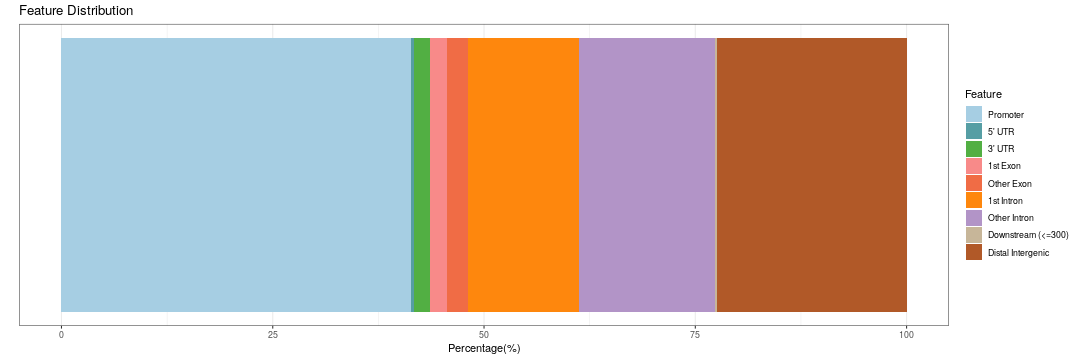
```

![](ChIPseq_In_Bioconductor2_files/figure-html/unnamed-chunk-33-1.png)

---
## Vizualising peak annotation

Similarly we can plot the distribution of peaks around TSS sites.

```r
plotDistToTSS(peakAnno)
```

![](imgs/TSS1.png)

---
# Vizualising peak annotation

ChIPseeker can also offer a succinct plot to describe the overlap between annotations.

```r
upsetplot(peakAnno, vennpie = F)
```

![](ChIPseq_In_Bioconductor2_files/figure-html/unnamed-chunk-35-1.png)

---
## Time for an exercise!

Exercise on ChIP-seq data can be found [here](../../exercises/exercises/chipseq_part2_exercise.html)

---
## Answers to exercise

Answers can be found [here](../../exercises/answers/chipseq_part2_answers.html)

R code for solutions can be found [here](../../exercises/answers/chipseq_part2_answers.R)