Epigenomics, Session 1

class: middle, inverse, title-slide

.title[
# Epigenomics, Session 1
]
.subtitle[
## <html><br />
<br />
<hr color='#EB811B' size=1px width=796px><br />
</html><br />
Bioinformatics Resource Center - Rockefeller University
]
.author[
### <a href="http://rockefelleruniversity.github.io/ATAC.Cut-Run.ChIP/" class="uri">http://rockefelleruniversity.github.io/ATAC.Cut-Run.ChIP/</a>
]
.author[
### <a href="mailto:brc@rockefeller.edu" class="email">brc@rockefeller.edu</a>
]

---

## Overview

- [Set up](https://rockefelleruniversity.github.io/ATAC.Cut-Run.ChIP/presentations/singlepage/Session1.html#set-up)
- [Epigenomic Approaches](https://rockefelleruniversity.github.io/ATAC.Cut-Run.ChIP/presentations/singlepage/Session1.html#epigenomic-approaches)
- [Fastq QC](https://rockefelleruniversity.github.io/ATAC.Cut-Run.ChIP/presentations/singlepage/Session1.html#fastq-qc)
- [FastP](https://rockefelleruniversity.github.io/ATAC.Cut-Run.ChIP/presentations/singlepage/Session1.html#fastp)

---
class: inverse, center, middle

# Set Up

---

## Materials

All prerequisites, links to material and slides for this course can be found on github.

* [ATAC.Cut-Run.ChIP](https://github.com/RockefellerUniversity/ATAC.Cut-Run.ChIP/)

Or can be downloaded as a zip archive from here.

* [Download zip](https://github.com/RockefellerUniversity/ATAC.Cut-Run.ChIP/archive/master.zip)

---
## Course materials

Once the zip file in unarchived. All presentations as HTML slides and pages, their R code and HTML practical sheets will be available in the directories underneath.

* **r_course/presentations/slides/**
Presentations as an HTML slide show.
* **r_course/presentations/singlepage/** 
Presentations as an HTML single page.
* **r_course/presentations/r_code/**
R code in presentations.
* **r_course/exercises/**
Practicals as HTML pages. 
* **r_course/answers/**
Practicals with answers as HTML pages and R code solutions.

---
## Set the Working directory

Before running any of the code in the practicals or slides we need to set the working directory to the folder we unarchived.

You may navigate to the unarchived ATAC.Cut-Run.ChIP-master folder in the Rstudio menu.

**Session -> Set Working Directory -> Choose Directory**

or in the console.

``` r
setwd("/PathToMyDownload/ATAC.Cut-Run.ChIP-master/r_course")
# e.g. setwd('~/Downloads/ATAC.Cut-Run.ChIP-master/r_course')
```

---
class: inverse, center, middle

# Epigenomic Approaches

---

## Epigenomic Approaches

There are a variety of genomics techniques to start to profile the epigenome of cells.

They fit a few different classes:

TF-bound/Histone Modifications: Cut and Run, Cut and Tag, ChIP-seq

Open Regions: ATAC-seq, MNase-seq and DNase-seq

Genome organization - Hi-C, HiCAR, Capture-C

---
## TF-bound/Histone Modifications

[(Oker, et al, 2020)](https://www.nature.com/articles/s41596-020-0373-x)

---
## TF-bound/Histone Modifications

* ChIP-seq
  - Strengths: Well established and validated across labs with robust antibody catalogs.
  - Weakness: High background, large cell input, potential artifacts from crosslinking/sonication, longest workflow.

* Cut & Run
  - Strengths: High signal-to-noise ratio, low input required (100 to 100,000 cells/nuclei), good resolution (20-80bp), can be used with crosslinking for weak/transient interactions, fewer reads (3-8 million).
  - Weakness: Sensitive to sample quality and nuclei preparation.

* Cut & Tag
	- Strengths: Highest signal-to-noise ratio, low input required (100 to 100,000 cells/nuclei), highest resolution (5-30bp), fewest reads (2 million).
	-	Weakness: The Tn5 bias toward open chromatin possible and GC, can't be used with crosslinking so can be tricky with transient TFs.

---
## Open Regions

* DNaseseq - Enzymatic digestion to extract signal from open chromatin around transcription factor binding sites.

* MNaseseq - Enzymatic digestion to extract signal repesenting nucleosome positioning.

* ATACseq - Uses transposases and offers a method to simultaneously extract signal from transcription factors binding sites and nucleosome positions from a single sample.

---
## ATACseq

ATACseq (Assay for Transposase-Accessible Chromatin using sequencing) uses a transposase to efficiently fragment accessible DNA prior to sequencing. The result provides a method to map the accessible/open chromatin genome wide.

In contrast to other techniques, ATACseq has several advantages including

* Low input material required (> 10,000 cells)
* Rapid experiment protocol (~ 4 hrs.)

---
## An overlaping workflow

Despite being different technologies that reveal differing biological phenomena the braod. strokes for analysis of all these techniques is the same:

1. Fastq QC. 
2. Alignment. 
3. Peak calling. 
4. Technique QC. 
5. Consensus Building. 
6. Counting. 
7. Differentials.

We will review analysis of these data types with a unified approach, but highlight key differences that need to be considered between technologies as we go.

---
class: inverse, center, middle

# Fastq QC

---

## The data

Our raw sequencing data will be in FASTQ format.

---
## The data

For your own data you will typically receive a fastq from the genomics group you are working with.

For published data the fastq will be available on GEO/SRA or ENA. For example we will be working today with data from the Fuchs lab: [*The pioneer factor SOX9 competes for epigenetic factors to switch stem cell fates*](https://www.nature.com/articles/s41556-023-01184-y)

For more information on the data you can look at [GEO](https://www.ncbi.nlm.nih.gov/geo/query/acc.cgi?acc=GSE208072) or download the fastq files (if you want) directly from ENA:

1. [Cut and Run](https://www.ebi.ac.uk/ena/browser/view/PRJNA858098). 
2. [ATAC](https://www.ebi.ac.uk/ena/browser/view/PRJNA858100).

We will work through how to run these early steps, but we will also provide intermediate files once we have completed some of the heavy processing as some of these steps will take too long to run in these sessions.

---
## Why QC?

At this time we will want to review the QC of our data. We can look for features like:

* Lack of library complexity
* Adapter contamination
* Poor sequencing quality

---
## How to QC

There are two main approaches:

1) Import the fastq into R and directly check metrics.

2) Use QC software like [fastp](https://github.com/OpenGene/fastp) or [FastQC](https://github.com/s-andrews/FastQC).

---
## Working with raw epigenomics data

Once we have downloaded the raw FASTQ data we can use the [ShortRead package](https://bioconductor.org/packages/release/bioc/html/ShortRead.html) to review our sequence data quality.

We have more detailed course material on how to work with raw sequencing data in the [**FASTQ in Bioconductor** session.](https://rockefelleruniversity.github.io/Bioconductor_Introduction/presentations/slides/FastQInBioconductor.html#1)

First we load the [ShortRead library.](https://bioconductor.org/packages/release/bioc/html/ShortRead.html)

``` r
library(ShortRead)
```

---
## Working with raw data

First we will review the raw sequencing reads using functions in the [ShortRead package.](https://bioconductor.org/packages/release/bioc/html/ShortRead.html)

We do not need to review all reads in the file to can gain an understanding of data quality. We can simply review a subsample of the reads and save ourselves some time and memory.

Note when we subsample we retrieve random reads from across the entire FASTQ file. This is important as FASTQ files are often ordered by their position on the sequencer.

---
## Reading a subsample

We can subsample from a FASTQ file using functions in **ShortRead** package.

Here we use the [**FastqSampler** and **yield** function](https://rockefelleruniversity.github.io/Bioconductor_Introduction/presentations/slides/FastQInBioconductor.html#41) to randomly sample a defined number of reads from a FASTQ file. Here we subsample 1 million reads. This should be enough to have an understanding of the quality of the data.

*NOTE: This step may take a little time, so you can skip it for now if you want.*

``` r
fqSample <- FastqSampler("~/Downloads/SOX9CNR_D0_rep1_R1.fastq.gz", n = 10^6)
fastq <- yield(fqSample)
```

---
## Reading a subsample

We have provided a subsampled version of our fastq file here for you to read in directly.

``` r
fastq <- readFastq(dirPath = "data/SOX9CNR_D0_rep1_R1_subsample.fastq.gz")
```

---
## Working with raw epigenomics data

The resulting object is a [ShortReadQ object](https://rockefelleruniversity.github.io/Bioconductor_Introduction/presentations/slides/FastQInBioconductor.html#10) showing information on the number of cycles, base pairs in reads, and number of reads in memory.

``` r
fastq
```

```
## class: ShortReadQ
## length: 1000000 reads; width: 40 cycles
```

---

## Raw epigenomics data QC

If we wished, we can assess information from the FASTQ file using [accessor functions.](https://rockefelleruniversity.github.io/Bioconductor_Introduction/presentations/slides/FastQInBioconductor.html#15)

* **sread()** - Retrieve sequence of reads.
* **quality()** - Retrieve quality of reads as ASCII scores.
* **id()** - Retrieve IDs of reads.

``` r
readSequences <- sread(fastq)
readQuality <- quality(fastq)
readIDs <- id(fastq)
readSequences
```

```
## DNAStringSet object of length 1000000:
##           width seq
##       [1]    40 CAACTGAATTTAGATAGGGAAGTAGCAGAAGGTTACATCT
##       [2]    40 AGGTTTTTGGGGTAAAATGCTCGCATAAATGACGGATCCC
##       [3]    40 CACTTCGTCTGCCAGCGGCGCAACGGCGTGGCGATGCCGG
##       [4]    40 TCTGAGCTCATCGTAAGAAGGCATGGCAGCAAGGGTGTGG
##       [5]    40 TCAGCTGTGGTGTGAGCTGCTTGCAAAAACATCGTGCTAG
##       ...   ... ...
##  [999996]    40 GTACGTTAAAACAGCTGTTACACATGGATCTATGCACTTA
##  [999997]    40 GTGAGAGGGTGCGCCAGAGAACCTGACAGCTTCTGGAACA
##  [999998]    40 GAAGCTGTGTCATATGTCATGCTCTGGTTAAAGGTTAACT
##  [999999]    40 TAGAGATGAAACCCATGTCTCAGAGCTCTTTCCTTCACAT
## [1000000]    40 TTGCATACATTAACTGGCTTGAGGTAACTATTATTTTTCC
```

---
## Base frequency with raw data

We can review the occurrence of DNA bases within reads and well as the occurrence of DNA bases across sequencing cycles using the [**alphabetFrequency()**](https://rockefelleruniversity.github.io/Bioconductor_Introduction/presentations/slides/FastQInBioconductor.html#18) and [**alphabetByCycle()**](https://rockefelleruniversity.github.io/Bioconductor_Introduction/presentations/slides/FastQInBioconductor.html#30) functions respectively.

Here we check the overall frequency of **A, G, C, T and N (unknown bases)** in our sequence reads.

``` r
readSequences <- sread(fastq)
readSequences_AlpFreq <- alphabetFrequency(readSequences)
readSequences_AlpFreq[1:3, ]
```

```
##       A  C  G  T M R W S Y K V H D B N - + .
## [1,] 15  5 10 10 0 0 0 0 0 0 0 0 0 0 0 0 0 0
## [2,] 11  7 11 11 0 0 0 0 0 0 0 0 0 0 0 0 0 0
## [3,]  5 14 15  6 0 0 0 0 0 0 0 0 0 0 0 0 0 0
```

---
## Base frequency with raw data

Once we have the frequency of DNA bases in our sequence reads we can retrieve the sum across all reads.

``` r
summed__AlpFreq <- colSums(readSequences_AlpFreq)
summed__AlpFreq[c("A", "C", "G", "T", "N")]
```

```
##        A        C        G        T        N 
## 11744925  8497685  8344368 11412114      908
```

---
## Assess by cycle with raw data

We can review DNA base occurrence by cycle using the [**alphabetByCycle()** function.](https://rockefelleruniversity.github.io/Bioconductor_Introduction/presentations/slides/FastQInBioconductor.html#30)

``` r
readSequences_AlpbyCycle <- alphabetByCycle(readSequences)
readSequences_AlpbyCycle[1:4, 1:10]
```

```
##         cycle
## alphabet   [,1]   [,2]   [,3]   [,4]   [,5]   [,6]   [,7]   [,8]   [,9]  [,10]
##        A 336004 302683 305045 291736 297843 287897 303525 294275 277613 295295
##        C 233900 185367 210355 230639 215323 211798 205233 208795 205654 207707
##        G 174963 239691 197263 197345 207617 212597 205342 192901 212591 207859
##        T 254822 272252 287337 280280 279217 287564 285893 304026 304142 289135
```

---

## Assess by cycle with raw epigenomics data

We often plot this to visualize the base occurrence over cycles to observe any bias.
First we arrange the base frequency into a data frame.

``` r
AFreq <- readSequences_AlpbyCycle["A", ]
CFreq <- readSequences_AlpbyCycle["C", ]
GFreq <- readSequences_AlpbyCycle["G", ]
TFreq <- readSequences_AlpbyCycle["T", ]
toPlot <- data.frame(Count = c(AFreq, CFreq, GFreq, TFreq), Cycle = rep(1:40, 4),
    Base = rep(c("A", "C", "G", "T"), each = 40))
```

---

## Assess by cycle with raw epigenomics data

Now we can plot the frequencies using ggplot2

``` r
library(ggplot2)
ggplot(toPlot, aes(y = Count, x = Cycle, colour = Base)) + geom_line() + theme_bw()
```

``` r
library(ggplot2)
ggplot(toPlot, aes(y = Count, x = Cycle, colour = Base)) + geom_line() + ylim(150000,
    350000) + theme_bw()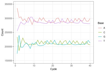
```

![](Session1_files/figure-html/mycRep1ReadsAlpByCyclePlot3-1.png)

---
## Quality with raw epigenomics data

We can also check some the reads' quality scores for our subsampled FASTQ data.

We use the [**alphabetScore()** function with our read's qualitys](https://rockefelleruniversity.github.io/Bioconductor_Introduction/presentations/slides/FastQInBioconductor.html#28) to retrieve the sum quality for every read from our subsample.

``` r
readQuality <- quality(fastq)
readQualities <- alphabetScore(readQuality)
readQualities[1:10]
```

```
##  [1] 1200 1200 1200 1200 1200 1200 1200 1200 1200 1200
```

---
## Quality with raw epigenomics data

We can then produce a histogram of quality scores to get a better understanding of the distribution of scores.

``` r
toPlot <- data.frame(ReadQ = readQualities)
ggplot(toPlot, aes(x = ReadQ)) + geom_histogram() + theme_minimal()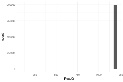
```

![](Session1_files/figure-html/mycRep1ReadsQScoresPlot-1.png)

---
## Quality Assessment

In this case the distribution of reads quality scores is a little strange. Normally we see a wider range of scores. This is likely due to some kind of loss of information during some transfer/conversion.

For a more in-detail review of working with fastqs in R you can check [here](https://rockefelleruniversity.github.io/Bioconductor_Introduction/presentations/singlepage/FastQInBioconductor.html). This also includes how to run filters on the data based on quality.

Most of the time we will not read in our fastqs. We normally only do this if there is a clear issue that we need to take a deep dive on. Instead use software like FastP to do a comprehensive FastQ review in one simple command.

---
## Fastp

This is one of the most popular and respected QC tools around.

It does what many of the others do, but it is VERY fast. There is a wrapper in R (developed by our team) so we can run it form R with ease: [Rfastp](https://www.bioconductor.org/packages/release/bioc/html/Rfastp.html)

There are many ways to customize including trimming options, barcodes and stringency. It will also handle the paired-end data simultaneously for us.

---
## Rfastp

- Trims low-quality bases from the 5′ and 3′ ends using a sliding window approach

- Automatically detects and removes adapters

- Corrects mismatched bases in overlapping regions of paired-end reads (based on quality)

- Trims polyA/polyX tails from the 3′ ends, depending on library type

- Filters out low-quality reads based on user-defined thresholds

---
## Rfastp

To run Rfastp we simply provide our two fastq files (or just one if we are running single end). We will also provide a name for the filtered Fastq file which is output.

``` r
library(Rfastp)
```

```
## Warning: package 'Rfastp' was built under R version 4.4.1
```

```
## Rfastp is a wrapper of fastp project: https://github.com/OpenGene/fastp
## 
## Please cite fastp in your publication:
## Shifu Chen, Yanqing Zhou, Yaru Chen, Jia Gu; fastp: an ultra-fast all-in-one 
##     FASTQ preprocessor, Bioinformatics, Volume 34, Issue 17, 1 September 2018,
##     Pages i884-i890, https://doi.org/10.1093/bioinformatics/bty560
```

``` r
rfastp_res <- rfastp(read1 = "/Users/mattpaul/Downloads/SRR20110418_1.fastq.gz",
    read2 = "/Users/mattpaul/Downloads/SRR20110418_2.fastq.gz", outputFastq = "SOX9CNR_D0_rep1_filtered")
```

---
## Rfastp QC results

Running RfastP creates several files:

1. XXX_R1.fastq.gz - FASTQ with poor quality reads filtered out
2. XXX.html - HTML file contains a QC report
3. XXX.json - JSON file with all the summary statistics

We can review the QC of our samples by checking out the *html* file. We have uploaded the result for this [here](data/SOX9CNR_D0_rep1_filtered.html)

You can also review the samples computationally using the *.json* file.

[Here](data/myc.html) is a second example report from a ChIPseq experiment of Myc from [ENCODE](https://www.encodeproject.org/experiments/ENCSR000EUA/).

---
## What to check?

* Quality
* Base Content
* Sequence over-representation (Kmer)
* Adapter content
* Duplicates

Whenever considering QC we rarely rule samples out at this early stage. But we keep an eye out for consistency between samples and if any sample looks bad across multiple metrics.

Always also consider your experiment, and previous experiments that may be similar.

---
## Rfastp QC plots

We can also look at some of the plots and QC metrics in R using the assigned object.

We have saved this in the data folder for you to load in *data/fastp_res.RData*.

``` r
load("data/fastp_res.RData")
```

``` r
qcSummary(rfastp_res)
```

```
##                      Before_QC     After_QC
## total_reads       1.745457e+08 1.705088e+08
## total_bases       6.981829e+09 6.801466e+09
## q20_bases         6.934319e+09 6.801466e+09
## q30_bases         6.934319e+09 6.801466e+09
## q20_rate          9.931950e-01 1.000000e+00
## q30_rate          9.931950e-01 1.000000e+00
## read1_mean_length 4.000000e+01 3.900000e+01
## read2_mean_length 4.000000e+01 3.900000e+01
## gc_content        4.239230e-01 4.193530e-01
```

---
## Rfastp QC plots

``` r
curvePlot(rfastp_res, curve = "content_curves")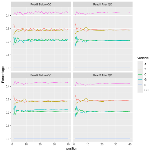
```

![](Session1_files/figure-html/unnamed-chunk-14-1.png)

---
## Rfastp options

We typically use the default settings, but there are lots of options to control Rfastp. Specifically this could help more stringent filtering if you observe any QC problems i.e. minReadLength or qualityFilterPercent.

---
## Example of custom filter usage

- Data from: ftp://ftp.sra.ebi.ac.uk/vol1/fastq/ERR458/ERR458755/ERR458755.fastq.gz or load from data folder.

*NOTE - this is single-end RNAseq, but for this example it doesn't matter*

``` r
rfastp_res <- rfastp(read1 = "data/ERR458755.fastq.gz", outputFastq = "ERR458755_rfastp")
```

---

## Rfastp - Base Quality

The quality score dips pretty low at the start of our reads.

``` r
curvePlot(rfastp_res)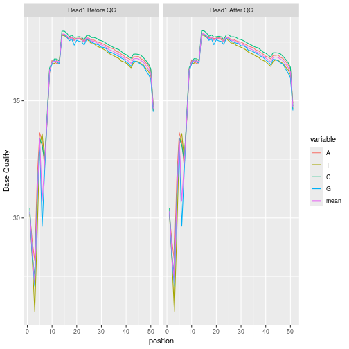
```

![](Session1_files/figure-html/unnamed-chunk-16-1.png)

---
## Rfastp - GC content
 
- N content indicates low confidence when calling bases
- GC content is higher at the front end of the read

``` r
curvePlot(rfastp_res, curve = "content_curves")
```

![](Session1_files/figure-html/unnamed-chunk-17-1.png)

---

## Adding filters

- Let's filter out the first 10 bases using "trimFrontRead1"

``` r
json_report <- rfastp(read1 = "data/ERR458755.fastq.gz", outputFastq = "ERR458755_rfastp",
    trimFrontRead1 = 10)
```

---

## Rfastp - Base Quality

- Notice low quality bases are eliminated at the start

``` r
curvePlot(json_report)
```

![](Session1_files/figure-html/unnamed-chunk-19-1.png)

---
## Rfastp - GC content
 
Trimming removes low-quality bases and ambiguous N bases, which can skew GC content at the 5′ end of reads

- This can normalize GC distribution, improving downstream alignment and quantification

What threshold defines abnormal GC content?
  - No strict cutoff — depends on organism, library prep, and sequencing platform

``` r
curvePlot(json_report, curve = "content_curves")
```

![](Session1_files/figure-html/unnamed-chunk-20-1.png)

---
## Time for an exercise!

Exercises for working with fastqs can be found [here](https://rockefelleruniversity.github.io/ATAC.Cut-Run.ChIP/exercises/exercises/MyExercise1_exercise.html)

---
## Answers to exercise

Answers can be found [here](https://rockefelleruniversity.github.io/ATAC.Cut-Run.ChIP/exercises/answers/MyExercise1_answers.html)

---
## References

* [ShortRead package.](https://bioconductor.org/packages/release/bioc/html/ShortRead.html) 
* [Rfastp](https://www.bioconductor.org/packages/release/bioc/html/Rfastp.html)